Similarity explanation
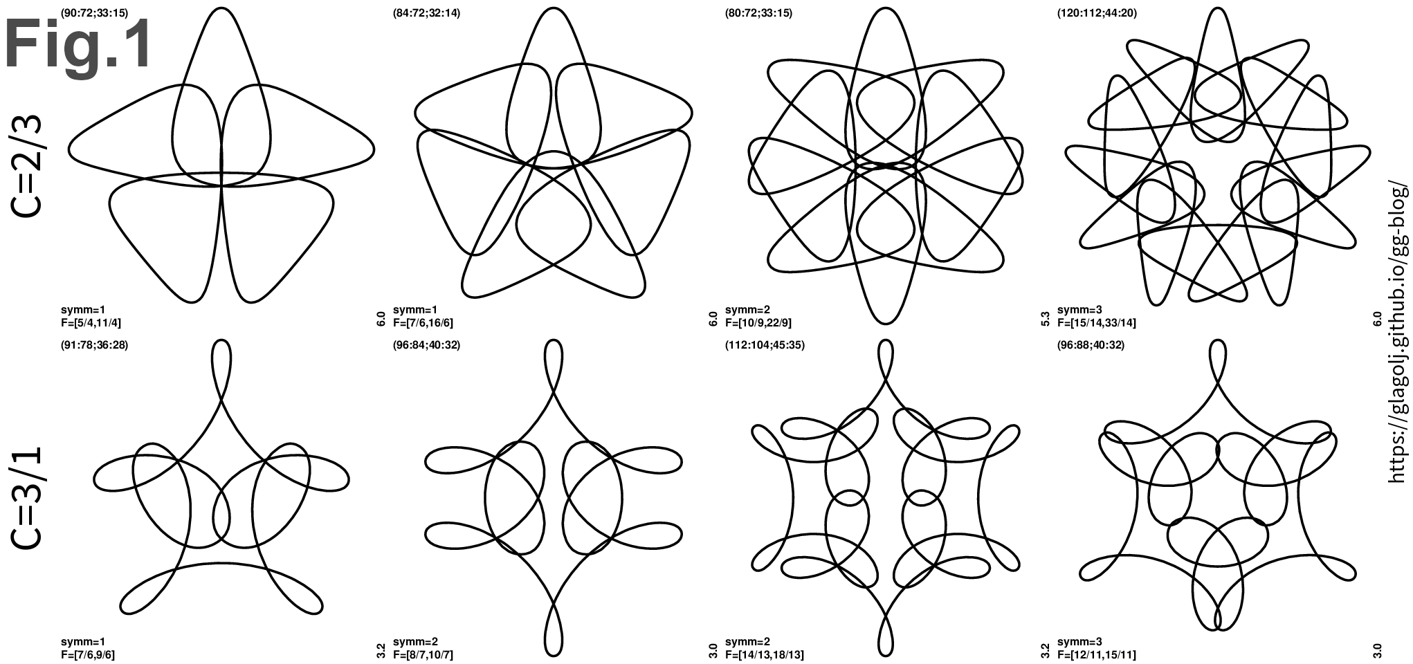
The 2nd order roulette curves are truly wild. And one thing that I stumbled upon are strong similarities between some of the gear-in-hoop-in-wheel spirograph patterns. This article is my attempt at explaining why are the top panels in Fig.1 (click for large version) all similar in a way, and what sets them apart from bottom panels.
Thematically this article is “theory #2”, while “theory #1” presented derivation of the parametric 2nd order roulette curves and their basic properties. I will continue to use the same notation here.
For TLDR: well, math is bit weird, but it is my attempt to explain additional commensurability behind Fig.1. I think that one can grasp the idea behind it solely looking at the plots, or my youtube video.
1 Useful equations and alternative approach
This section is a bit of a detour. It contains additional useful equations that I found in the meanwhile, but I didn’t know where else to fit them. While I didn’t formally derive every single equation in this article, I did check all expression using battery of 25,000 numerical examples.
Let us first repeat the basic expressions. A 2nd order roulette \((n_0:n_1;n_2:n_3)\) has 3 cogs in total: The \(n_0\) teeth outer wheel is stationary and contains a hoop \((n_1;n_2)\) with \(n_1\) outside and \(n_2\) interior teeth. Inside the hoop we have a small gear with \(n_3\) teth with a hole for the pen. The resulting curve is governed with 2 fundamental ratios, or frequencies \(F=(f_0,f_1)\) where \(f_0 = {n_0}/{n_1}\) and \(f_1 = {n_0 \, n_2}/({n_1 \, n_3})\). The two frequencies are connected to the total number of turns each gear makes: \(F=(T_1/T,T_3/T)\), where \(T\) is number of turns inside the big stationary \(n_0\) wheel, \(T_1\) is number of hoop turns, and \(T_3\) is the number of smallest gear turns. And the number of rotational symmetries is \(n_{\rm symm} = {\rm gcd}( T_1, T_3 )\). Note that my phrase turn is not the same as rotation. For an example \(T\) counts how many \(360^\circ\) the polar angle \(t\) travels in total. In contrast the total rotation of the hoop is \(t-t_1\), and \(T-T_1\) will be total number of full \(360^\circ\) rotations of the hoop.
One of the pioneering efforts at prediction of gear-in-hoop-in-wheel outcomes was done by u/HomegrownTomato on reddit. In short u/HomegrownTomato reduces two fractions \(n_1/n_0\) and \(n_3/n_2\) to their irreducible forms and then asks if in their product \((n_1/n_0)\cdot (n_3/n_2)\) the denominator of the 1st fraction is canceled with the numerator of the 2nd fraction. If yes the resulting curve is not rotationally symmetric (i.e. it is a “butterfly” or \(n_{\rm symm}=1\)). And if there is a partial cancellation of the factors, one gets reduced symmetry or “compression”. Apart from the inversion (\(n_1/n_0\) instead of \(n_0/n_1\)), that clearly resembles expressions I outlined in the 1st article. But here are alternative expressions that make closer match:
\[{T}/{n_{\rm symm}} = \frac{n_1 \; n_3}{n_0 \; {\rm gcd}(n_2,n_3)}, \tag{Eq.1.1}\] \[{T_1}/{n_{\rm symm}} = {n_3} / { {\rm gcd}(n_2,n_3) }, \tag{Eq.1.2}\] \[{T_3}/{n_{\rm symm}} = {n_2} / { {\rm gcd}(n_2,n_3) }. \tag{Eq.1.3}\]If-and-only-if the right hand side of (Eq.1.1) is an integer than the curve is a “butterfly” (\(n_{\rm symm}=1\)). And if-and-only-if it evaluates to a fraction, then the denominator is the number of rotational symmetries \(n_{\rm symm}\). However, if one needs a closed form expression we can use one of these two
\[{n_{\rm symm}} = \frac{ {\rm lcm} \bigl( n_0 \: {\rm gcd}(n_2,n_3), n_1 \: n_3 \bigr) }{ n_1 \; n_3 }, \tag{Eq.2.1}\]or
\[{n_{\rm symm}} = \frac{ n_0 }{ {\rm gcd} \bigl( n_0, n_1\:n_3 / {\rm gcd}(n_2,n_3) \bigr) }. \tag{Eq.2.2}\]The last equation is useful as it demonstrates that rotational symmetry is a factor of \(n_0\) that is not canceled by other gears.
2 Statement of the problem
The goal of this article is to explain Fig.1. Why are bottom panels all similar to each other, and what sets them apart from the top panels? The similarity itself is a weak property: for instance one can use cogs that are drastically different in size and then the semblance will be diminished. Nevertheless as demonstrated in Fig.1 the resemblance of the curves can be striking.
I stumbled upon the similarity sets by surveying 2nd order roulette curves. After seeing many plots it becomes apparent that there is some kind of repetition of patterns. The repetition looked quite regular, such as, in bunch of plots every 5th curve is kind of related. But then checking for different \({n_{\rm symm}}=4\) it looked like every 4th curve is alike. However not always, sometimes for \({n_{\rm symm}}=4\) it seemed like every 8th curve is similar. My next step was to try to formulate some linear formula for such hopping. It took a while, and astonishingly I did find a linear combination that works:
\[C = \frac{ T_1 - n_{\rm symm} (T_1 - T) }{T_3 - T_1}. \tag{Eq.3.1}\]The bottom panels if Fig.1 all have \(C=3\), while top panels produce \(C=2/3\). As long as different curves \(F=(T_1/T,T_3/T)\) yield the same value \(C\) they will look similar. Or somewhat similar. Better to say that they will have a common “theme”. The rule is sometimes broken, but it seems that for \(T_3<2T_1\) it rather holds (this is probably due to “roses and ropy” patterns).
That (Eq.3.1) works is additionally reinforced by observation that simpler fractions, such as \(C=2/1\), are connected to simpler curves, while for instance \(C=13/8\) curves all look more complex. The factors in \(C\) clearly measure something. Then the question is: Why does the question (Eq.3.1) work? Some additional commensurability is clearly at work. Before trying to answer that question let me put here an equivalent expression using teeth numbers \(n_x\):
\[C = \frac{n_3}{n_0} \cdot \frac{ n_0 - n_{\rm symm} (n_0 - n_1) }{n_2 - n_3}. \tag{Eq.3.2}\]3 Similarity components
The parameters \(T_x\) describe the main ratios or frequencies \(F=(f_0,f_1)\). I loosely use term frequency as one can view curve as a trajectory, and then the ratios are indeed frequencies. Thus (Eq.3.1) is a statement of some commensurability of some angles or orientations of the system. That sounds like a resonance of a physical system. To carry analogy further: at discrete points during the trajectory some angles repeatedly take value of integer multiple of \(360^\circ\) at the same time. Even before identifying which angles are involved we can ask how many times \(n_C\) that happens. This gives us number of components or segments. And at the ends of the segments special commensurability condition occurs. The result for \(n_C\) is analogous to the expression that gives us the number of rotational symmetries \(n_{\rm symm}={\rm gcd}(T_1,T_3)\) and reads
\[n_C = {\rm gcd} \Bigl( {T_3 - T_1} , { T_1 - n_{\rm symm} (T_1 - T) } \Bigr). \tag{Eq.4}\]I found at least two different ways how to start from (Eq.3.1) and arrive at (Eq.4), but the following explanation is, imho, simplest: The polar angles of cogs \(t\), \(t_1\), and \(t_3\) (see here) range in \(t\in [0,T*2\pi]\) or \(t_1\in [0,T_1*2\pi]\), thus the question how many times their linear combinations are simultaneously integer multiple of \(2\pi\) is then the above gcd expression. Important to note is that since both arguments of gcd function are divisible by \(n_{\rm symm}\), thus \(n_C\) is multiple of \(n_{\rm symm}\).
Fig.2 (click for large version) demonstrates how curves divide into \(n_C\) components. The curves have different rotational symmetries, from 1 to 3, while \(n_C\) ranges from 2 to 6, but \(C=3/1\). The plot contains all 3 bottom panels from Fig.1.
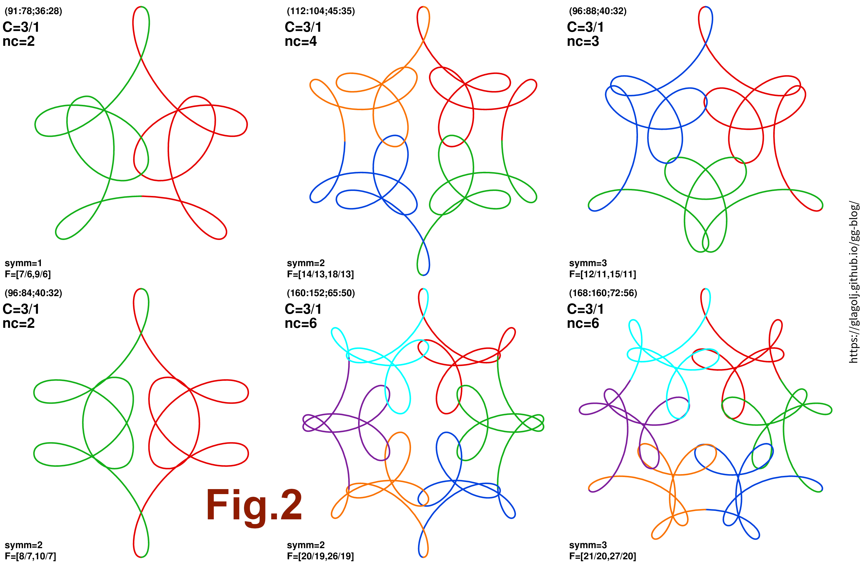
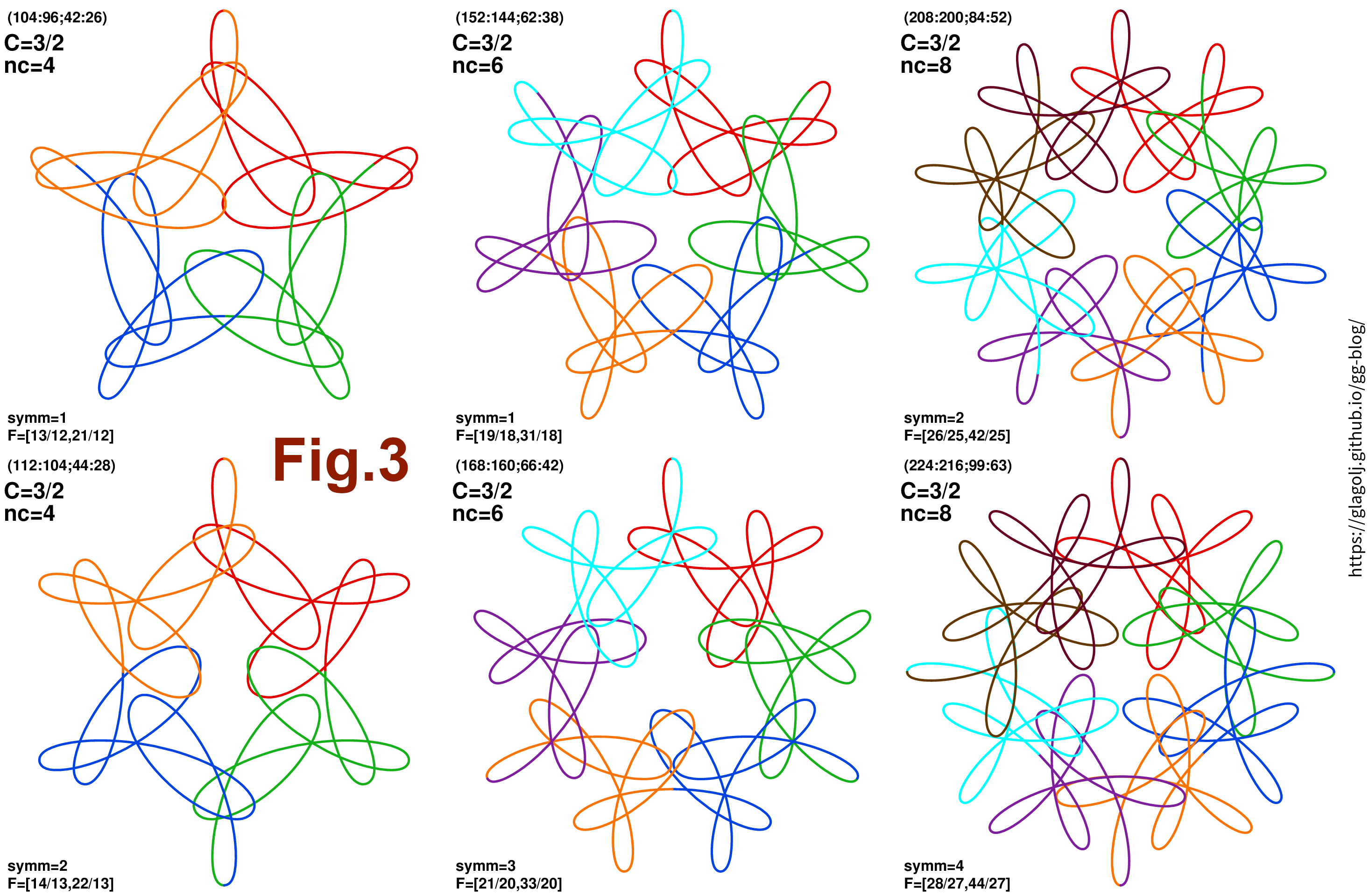
While the individual segments or components (both within the same curve and across curves) are not exactly the same, they do have a similar “theme” or “motif”: compare, for instance, the first segments in each panel (red line). Another example is shown in Fig.3 for \(C=3/2\). Rotational symmetry is 1 to 4, while number of components \(n_C\) takes values 4, 6, and 8. Compare red segments, or blue segments across each panel. Clearly there is a common theme on display. An interesting thing is that \(n_C\) is not necessarily the number of “arms” of the curve: top-left panel in Fig.3 has no rotational symmetry (\(n_{\rm symm}=1\)), yet to us it looks like a star with 5 arms, but actually is made from \(n_C=4\) components. And those 4 segments do indeed look very similar to each other. But together they form what looks to our eyes a 5-armed star.
4 Similarity parameterization
In order to proceed it is easier to parameterize (Eq.3.1). That is, we will solve it for \(T\), \(T_1\), and \(T_3\) that yield the same \(C\). The parameterization described here is bit different from what I used in previous articles, as this choice of variables has more immediate interpretation. First let us denote explicitely fraction \(C=C_p/C_q\) where \(C_p\) and \(C_q\) are mutually prime. Next we introduce \(m=T_1-T\) which is just a simple change of variables. Final step is to use \(n_C=l\cdot n_{\rm symm}\). This follows as both arguments in (Eq.4) are divisible by \(n_{\rm symm}\), thus \(n_C\) is multiple of \(n_{\rm symm}\). Next we observe from (Eq.3.1) and (Eq.4) that \(C_q n_C = T_3-T_1\) and \(C_p n_C = { T_1 - n_{\rm symm} (T_1 - T) }\). Or solving explicitely for \(T\), \(T_1\), and \(T_3\) gives all together
\[C = C_p / C_q, \tag{Eq.5.1}\] \[n_C = l \; n_{\rm symm}, \tag{Eq.5.2}\] \[T_1 = C_p \; l \; n_{\rm symm} + m \; n_{\rm symm} , \tag{Eq.5.3}\] \[T_3 = (C_p + C_q) \; l \; n_{\rm symm} + m \; n_{\rm symm} , \tag{Eq.5.4}\] \[T = C_p \; l \; n_{\rm symm} + m \; (n_{\rm symm} - 1), \tag{Eq.5.5}\]which doesn’t look any insightful. Yet. But it allows us to easily find curves \(F=(T_1/T,T_3/T)\) for given \(C=C_p/C_q\) and \(n_{\rm symm}\). To obtain teeth numbers \((n_0:n_1;n_2:n_3)\) one has to use frequency inversion. My javascript plotter can pefrom the inversion.
Parameters \(l\) and \(m\) are arbitrary positive integers. However not all possible values are allowed as we have to satisfy that gears physically fit into each other \(0<T<T_1<T_3\), their rotational symmetry \({\rm gcd}(T_1,T_3)=n_{\rm symm}\) and \({\rm gcd}(T,T_1,T_3)=1\). That still leaves \(\infty^2\) possibilities, but the resulting space \((m,l)\) looks like a swiss cheese with holes. Though few useful properties can be inferred:
\[{\rm gcd}(m,l)= {\rm gcd}(m,n_{\rm symm})= {\rm gcd}(m,n_C)= 1, \tag{Eq.6}\]and \({\rm gcd}(m,C_p)={\rm gcd}(T_1,T)\).
In previous articles I used different parameterization \((k,l)\) instead of \((m,l)\) as here. The connection is simple: \(k=l\cdot C_p+m\), but \(m\) has a direct meaning (later in text) and allowed me to solve the problem.
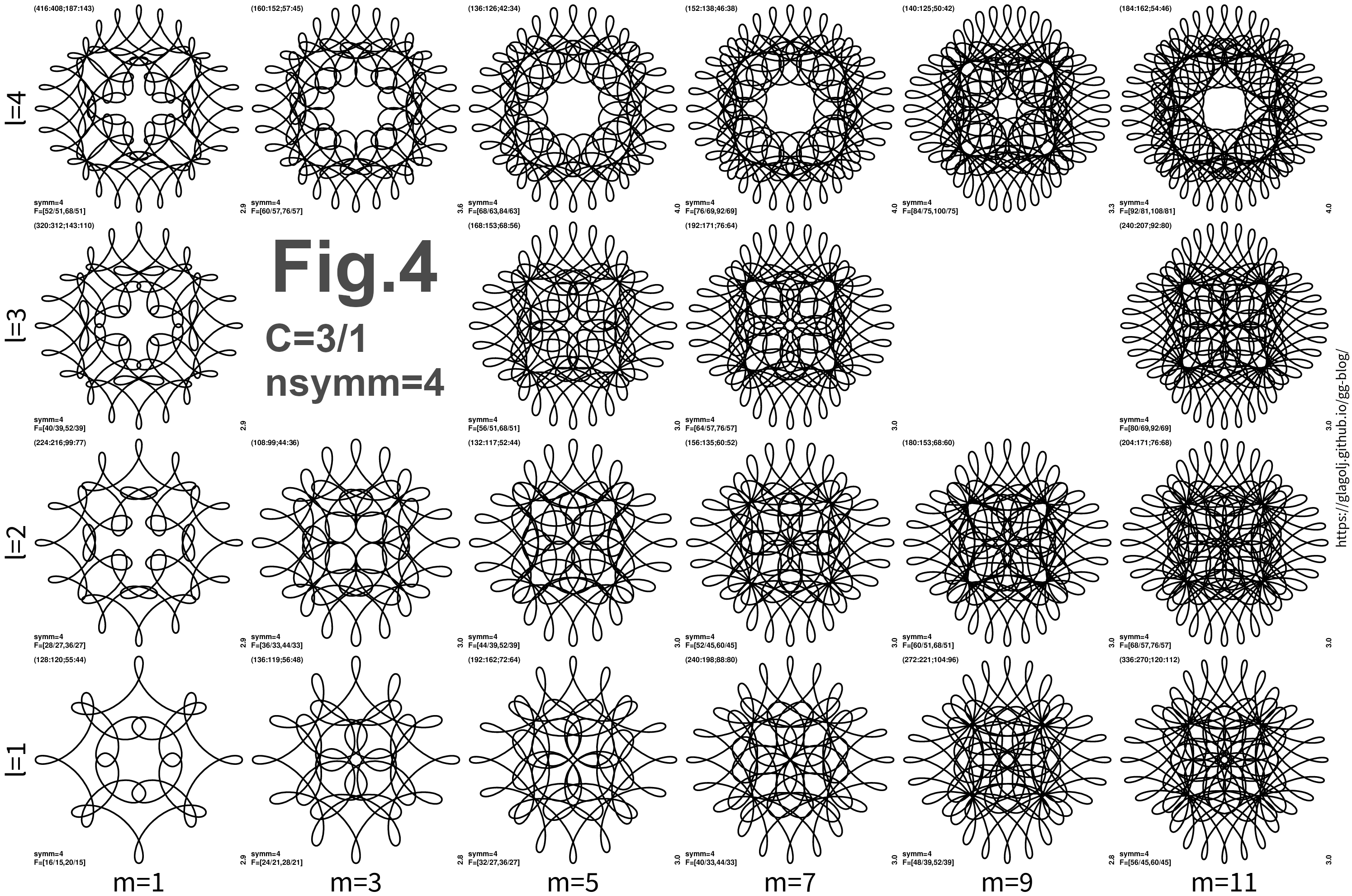
Fig.4 shows \((m,l)\) grid of patterns for \(n_{\rm symm}=4\) and \(C=3/1\). Similarity of patterns is quite striking. Notice that even values of \(m\) are missing, and (3,3) and (9,3) are also not possible.
5 Special orientation of gears
Final part of out effort is to examine what is exactly specially aligned at discrete points along the trajectory and why that matters. Starting point are polar angles \(t\), \(t_1\), \(t_2\), and \(t_3\) introduced in the original article. In short those are polar angles of \(n_0\), \(n_1\), \(n_2\) and \(n_3\) teethed surfaces, respectively. I will also make few simplifying assumptions. First is initial alignment \(\varphi_p=0\), as that makes expressions bit simpler and plots more striking. Second assumption is using \(t_2=t_1\) (which is (Eq.3.1) from theory #1). That makes all polar angle dependencies linear and by far easier to trace. However the similarity holds regardless of such linearity assumption (for instance Fig.4 uses (Eq.3.2) from theory #1).
Let us now examine \(i\)-th segment of the curve. In total we have \(n_C\) similar components. With linearity assumption we can denote the endpoints of \(i\)-th segment as:
\[t(i) = \frac{i}{n_C} \; T \; 2\pi, \tag{Eq.7}\]here \(i\) is an integer from \(0\) to \(n_C\) (and \(0\) and \(n_C\) connect). The equation comes from the range of polar angle \(t\in [0,T*2\pi]\), and using linearity assumption we split it into \(n_C\) segments. Figures 2 and 3 illustrate breaking the curve into components.
We will now examine two special angles \(t_1-t\) and \(t_3-t\). The angle \(t-t_1\) is the total rotation angle of the hoop \((n_1;n_2)\). In a similar way it is easy to see that \(t-t_3\) is the total rotation angle of the smallest cog \(n_3\) (and minus sign is not really important \(t_1-t\) vs \(t-t_1\)). Using polar angle equations \(t_1=f_0 t\), \(t_2=t_1\), and \(t_3=(n_2/n_3)t_2\), and parametrization (Eq.5.1-5.5) after some algebra we obtain the rotation angle of geared elements
\[\delta_C = 2 \pi / n_C, \tag{Eq.8.1}\] \[t_1(i) - t(i) = i \cdot m \cdot \delta_C \;\; {\rm mod} \;\; 2\pi, \tag{Eq.8.2}\] \[t_3(i) - t(i) = i \cdot m \cdot \delta_C \;\; {\rm mod} \;\; 2\pi. \tag{Eq.8.3}\]There is a lot to unpack from this result. The equations are finally simple and possible to interpret in physical terms, in contrast to rather opaque nature of (Eq.3.1). At the ends of the \(i\)-th segment orientations of both the hoop \((n_1;n_2)\) and the smallest gear \(n_3\) are the same. Moreover since \(m\) and \(n_C\) don’t share a common factor, see (Eq.6), the orientations form a perfect \(n_C\)-sided figure.
Another usefull expression is:
\[t(i) = i \cdot m \cdot (n_{\rm symm}-1) \cdot \delta_C \;\; {\rm mod} \;\; 2\pi. \tag{Eq.9}\]Polar angle \(t(i)\) describes position of the hoop within the static ring \(n_0\). In other words it is angle of the contact point between the two. In contrast to (Eq.8.1-8.3) factor \((n_{\rm symm}-1)\) can divide \(n_C\), meaning that \(t(i)\) only sometimes form \(n_C\)-sided figure. For curves without rotational symmetry (\(n_{\rm symm}=1\)) it is always 0, which means that the similarity is mostly driven by (Eq.8.1-8.3).
Final piece of information is how many \(360^\circ\) full circles do these angles span during each segment. Or what is the rest in (Eq.8.1-9) that modulo operation subtracted. We obtain:
\[\Bigl( t_1(i+1) - t(i+1) \Bigr) - \Bigl( t_1(i) - t(i) \Bigr) \propto 0, \tag{Eq.10.1}\] \[\Bigl( t_3(i+1) - t(i+1) \Bigr) - \Bigl( t_3(i) - t(i) \Bigr) \propto C_q \cdot 2\pi, \tag{Eq.10.2}\] \[t(i+1) - t(i) \propto C_p \cdot 2\pi. \tag{Eq.10.3}\]This gives us meaning of parameters \(C=C_p/C_q\). Therefore \(C_q\) is the number of times the smallest wheel \(n_3\) fully rotates during each segment. And \(C_p\) is how many times the contact point between the static ring \(n_0\) and the hoop \((n_1;n_2)\) turns around during each segment. This can be loosely viewed like a resonant condition \(C_p:C_q\), or how many times \(n_3\) fully rotates while hoop touch point turns around \(n_0\). Note that if we are counting by hand \(360^\circ\) turns while drawing on paper, we still have additional terms in (Eq.8.1-9), so counting will be easy only for \(m<l\).
Let us illustrate these findings with some examples. First consider only \(m=1\) as it is simplest to visualize. Then the orientations \(t_1(i) - t(i)\) and \(t_3(i) - t(i)\) of both movable cogs simply go through \(0\), \(\delta_C\), \(2\delta_C\), …, \(360^\circ\). During each segment, between \(i\) and \(i+1\) endpoints, cogs execute similar \(C_p:C_q\) motion. The wheels start from the same orientation and end in the same orientation. The motion of the geared elements in not exactly the same across different segments, but similar enough, and that gives appearance of similarly looking components. Same \(C\) across different curves means that their individual segments have same \(C_p:C_q\) motion and that looks to us as a kindred “theme” (Fig.4 or Fig.1).
Fig.5 illustrates position and orientation of cogs at the end of each segment for \(C=3/1\), \(n_C=6\), \(n_{\rm symm}=2\), \(m=1\), and \(l=3\). Dashed lines demonstrate the alignment of rotations from (Eq.8.1-8.3): \(60^\circ\), \(120^\circ\), \(180^\circ\), \(240^\circ\), \(300^\circ\), and \(0\) in the end. Note that the position of the smallest wheel \(n_3\) is not always at the top of the hoop, only that their orientations are the same. In this case the position of the hoop within the static wheel \(n_0\) also makes 6-fold figure, see (Eq.9).
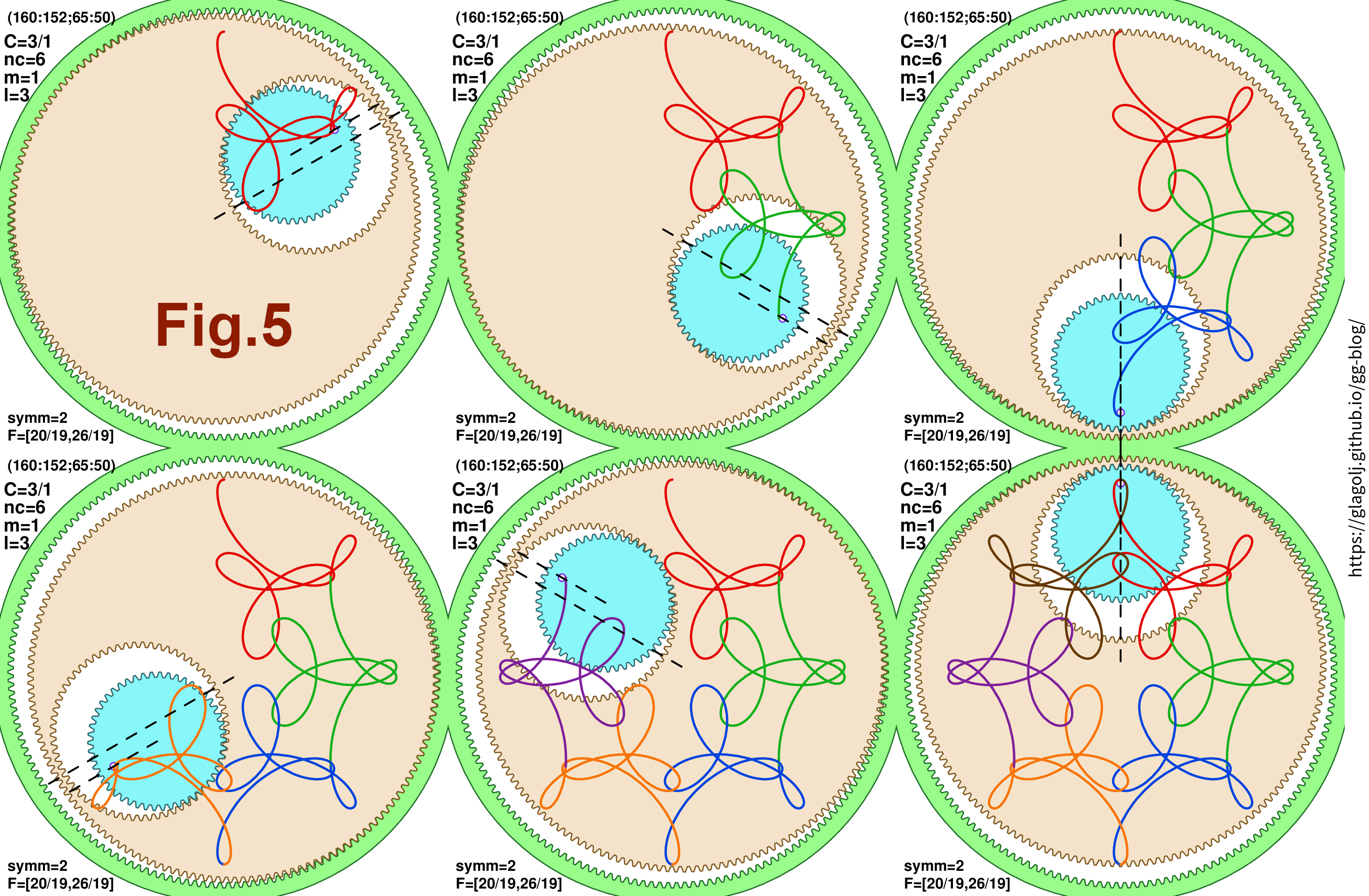
Fig.6 is very similar (in the plot we have \(C=3/1\), \(n_C=6\), \(n_{\rm symm}=1\), \(m=1\), and \(l=6\)). The segments in both Fig.5 and Fig.6 are similar looking, and that drives the overall resemblance between the two curves. Since Fig.6 uses \(n_{\rm symm}=1\) the hoop is always at the top of the wheel \(n_0\): (Eq.9) always produces 0 in this case, but that doesn’t impact overall impression.
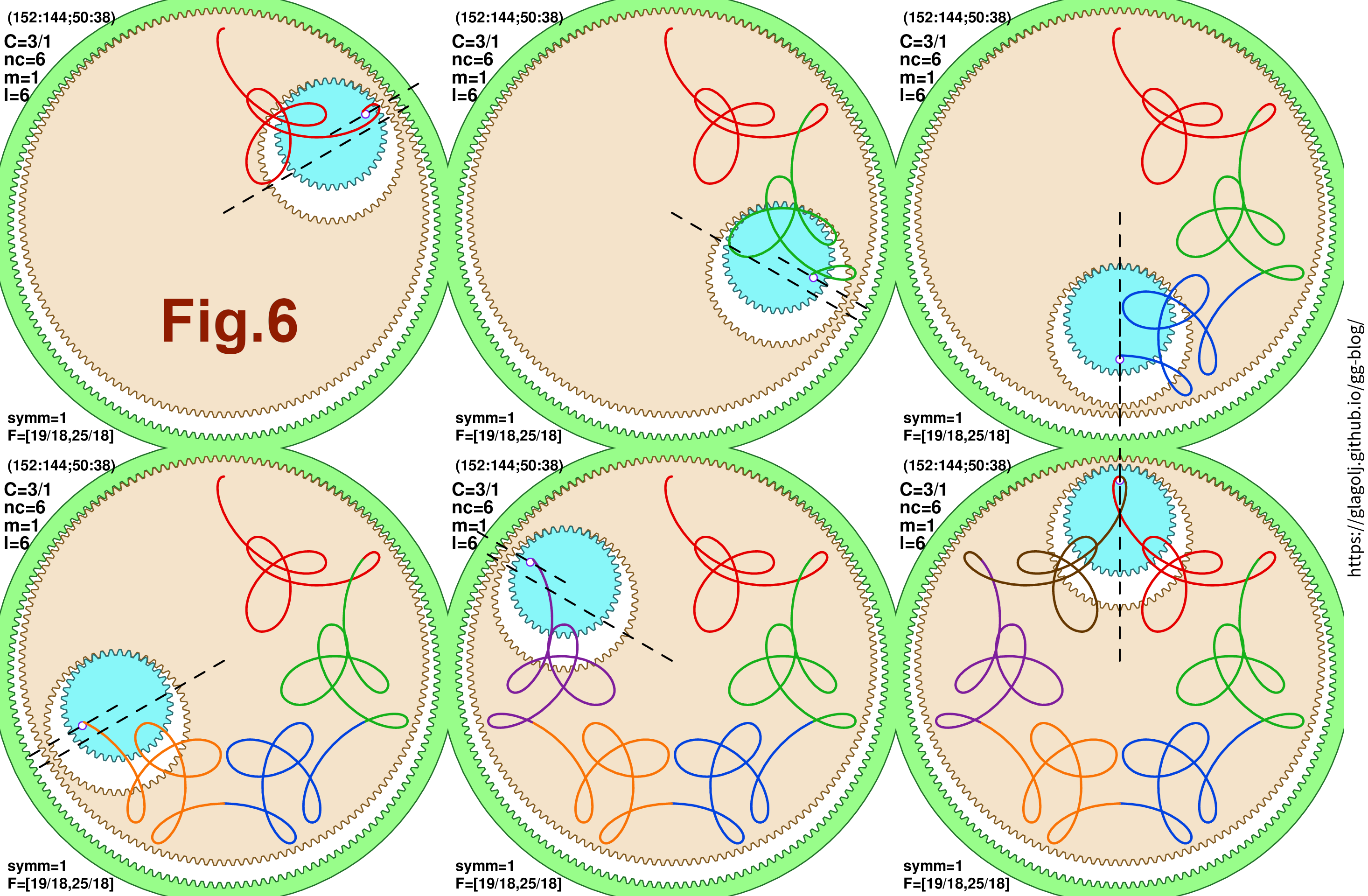
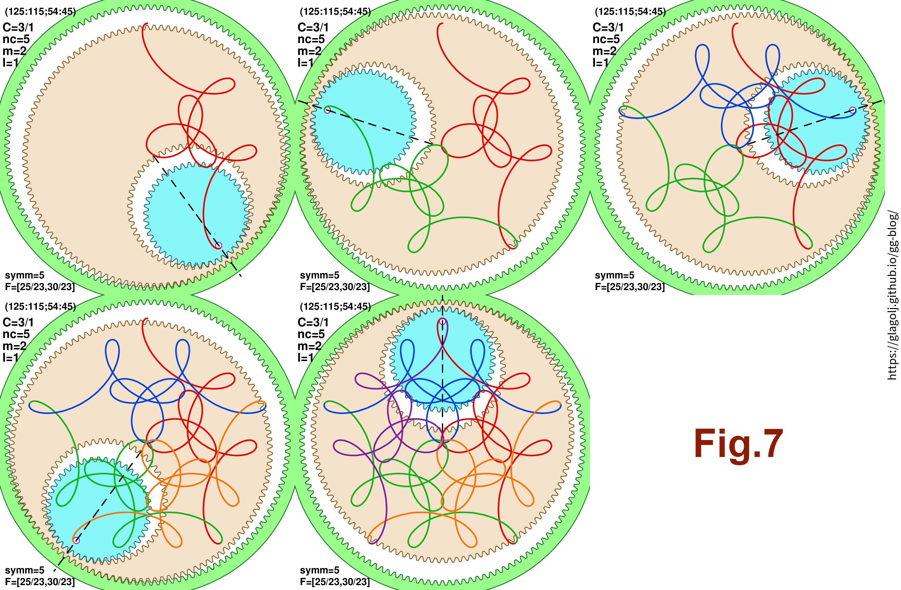
Fig.7 illustrates \(m>1\) (in the plot we have \(C=3/1\), \(n_C=5\), \(n_{\rm symm}=5\), \(m=2\), and \(l=1\)). In this case rotations of both hoop and smallest gear form 5-fold figure, but since \(m=2\) in this case rotation angles skip every second \(\delta_C=72^\circ\): at the end of the first segment we have \(2*72^\circ\equiv 144^\circ\), then \(4*72^\circ\equiv 288^\circ\), \(6*72^\circ\equiv 72^\circ\), \(8*72^\circ\equiv 216^\circ\), and finally \(10*72^\circ\equiv 0\). In general for \(m>1\) the lines from different passes will cross more and more.
I also prepared a youtube clip. The video shows pairs of similar curves drawn simultaneously. It is helpfull to see orientation alignment at the segments ends, and “similarity” of segments arising from \(C_p:C_q\) motion.
6 Zero or negative coefficient \(C\)
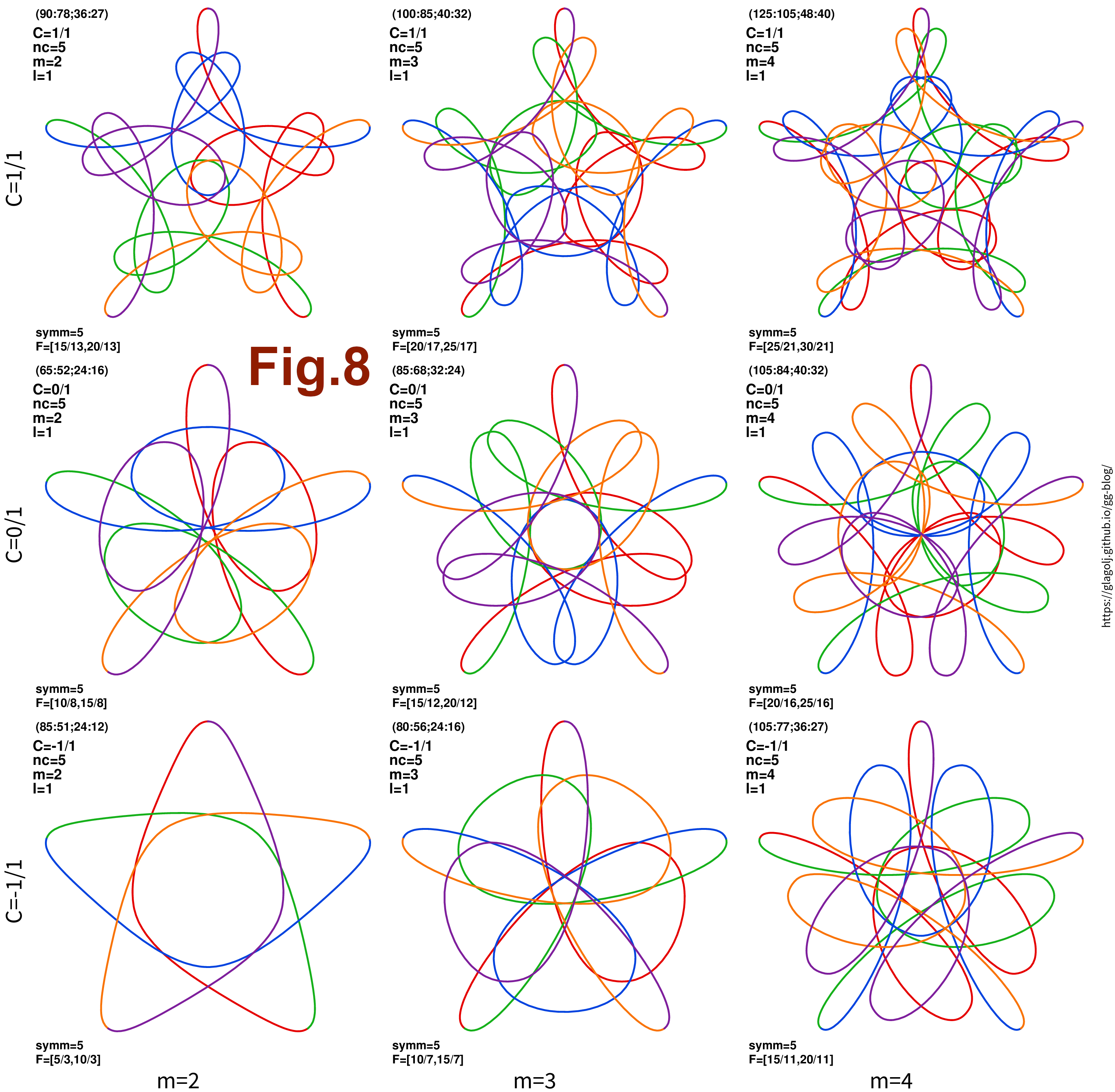
I have so far skirted the issue that coefficient \(C\) from (Eq.3.1) can have non-positive values. While the denominator is always positive, the numerator can be \(0\) or even negative. However for \(C\le 0\) the simple condition \(0<T<T_1<T_3\), that cogs physically fit into each other, is harder to satisfy, and when \(n_{\rm symm}=1\) it is not possible at all! Fig.8 shows some solutions and comparison between \(C=-1\), \(C=0\) and \(C=1\).
7 Summary
From previous articles I have a collection of about 500 interesting curves shown in two youtube slide-shows (here and here). While the collection is probably biased in some ways, it predates any work on “similarity” sets. It is interesting to check histograms of \(C=C_p/C_q\) and \((m,l)\) parameters. Not surprisingly the vast majority of curves have small numeric values of parameters, as such choice indicates simpler curves. The frequency of any parameter seems roughly inversely proportional to its absolute value. It is telling that out of all \((m,l)\) combinations in \(80\%\) of cases at least one of the two is equal to \(1\). About the sign of \(C\) I found: \(C>0\) in \(52\%\) of cases, \(C=0\) in \(25\%\), and \(C<0\) in \(23\%\) of examples.
I did a survey of curves for different \(C\) in one older article: link.
Parameters described here are not easy to use, and certainly it is not easy to find a match among acrylic Wild Gears to make pattern on paper. But on the other hand it is easy to find simple curves that have a “common theme”. All parameters are integers and have immediate meaning, and let me summarize it:
-
\(n_{\rm symm}\) is the number of rotational symmetries.
-
\(n_C\) is the number of components or segments. Gear orientations at the end of segments form \(n_C\)-fold figure.
-
\(l=n_C/n_{\rm symm}\) is number of segments per rotational degree.
-
\(m\) describes forming of \(n_C\)-fold figure: gear orientations go through every \(m\)-th position.
-
Along each segment the smallest gear \(n_3\) rotates \(C_q\) times \(360^\circ\).
-
The hoop makes \(C_p\) times full \(360^\circ\) turns along each segment. \(C_p\) can be positive, 0, or negative.
-
Similarity of segments comes from \(C_p:C_q\) condition, i.e. cogs execute similar (but not the same!) motions during each segment.
A way to compress this is to say that gear-in-hoop-in-wheel curves and their basic properties (like rotational symmetry) come from commensurability of teeth numbers (that is polar angles and their measures \(T\), \(T_1\) and \(T_3\)). But additionally there can be commensurability of gears physical rotations (measured with differences \(T_1-T\) and \(T_3-T\)) which then sorts patterns into similarity or affinity sets.
A small remaining puzzle is why, for instance, top-left panel in Fig.3 is a “butterfly” (\(n_{\rm symm}=1\)), has \(n_C=4\) segments, and yet to our eyes looks like a 5-armed star. I think that one could work bit more in the framework I described in this article (segments and their polar angles and rotations) and have a simple integer prediction of how many arms it will resemble. And just as I wrote the last two sentences I realized that \(1+4=5\): all curves in Fig.3 look like that \(n_{\rm arm}=n_{\rm symm}+n_C\) could work. But it is not too hard to come with some counterexamples…
On a personal note these similarity sets were very hard nut to crack. At each point the only advance I could make was only after I introduced a meaningful variable or parameter. Otherwise equations just stay long and opaque.