Second order roulette or gear-in-hoop-in-wheel spirograph
Spirograph is a fond toy for many people. But the result is soon exhausted, unless one starts to combine lines from different setups. In the last decade Aaron Bleackley managed to invigorate things with new geared toys called wild gears. The wild gears are produced with high precision and it is possible to use 3 elements in a gear-in-hoop-in-wheel combo that produces intriguing shapes on paper. This article presents a full parametric solution of the new curves and examines their properties. I also solved extensions for weird shapes and even higher orders, which produced a lot of crazy curves that I will slowly share on this blog.
As an introduction on how gear-in-hoop-in-wheel works I can offer my video with simulated cogs, or another video by spirographicart.com with the same setup using wild gears on paper.
About naming: Roulette is a general term for
rolling a curve on top of another
curve. Hypocycloids and epicycloids are specific
terms used for circles only, and don’t apply to triangles and
ovals. It seems to me that “higher order roulette” is an accurate name
for patterns obtained with gear-in-hoop-in-wheel, especially as it
also covers mounting gears on the outside instead of the inside, or adding more
gears, or triangular cogs instead of circular.
And it doesn’t sound bad.
Another term to discuss is “hoop”. Aaron Bleackley uses it exclusively
for the geared element with concentric inner and outer circle. But it
is the offseted, non-concentric, version that is crucial in production
of these new weird curves. I am not a native English speaker, but
googling “hoop” brings all kind of images and I think that
it is not too big stretch to call even offset version a hoop.
In TLDR case: consider at least two short sections “7 Simple numerical example” and “9 Gallery of curves and online plotter”.
1 Parametric equation
Lets start with ordinary spirograph \((n_0:n_1)\) which consists of a smaller gear with \(n_1\) teeth rolling inside a bigger static wheel with \(n_0\) teeth. The solution is the famous hypotrochoid parametric curve written here as a vector equation (compare with complex parametrization)
\[\begin{bmatrix} x \\ y \end{bmatrix} = \hat{R}(t) \begin{bmatrix} r_0 - r_1 \\ 0 \end{bmatrix} + \hat{R}(t - t_1) \begin{bmatrix} p*r_1 \\ 0 \end{bmatrix} \tag{Eq.1}\]where \(\hat{R}(\alpha)\) is a rotation matrix for angle \(\alpha\), radii are \(r_0=n_0\) and \(r_1=n_1\), while \(t_0=t\) and \(t_1\) are their polar angles. The rotation matrix product results in simple \([{\rm cos}(\alpha),{\rm sin}(\alpha)]\) terms. Pen-hole distance from the gear center is \(p*r_1\), while the scaled parameter \(p\) is in the range [0,1]. The only remaining unknown is connection between two polar angles \(t\) and \(t_1\). Since the circles are geared and do not slip, the paths along circumference are same \(r_0*t=r_1*t_1\), or \(t_1=(n_0/n_1)*t\). Note that the angle \(t-t_1\) is the total rotation angle of \(n_1\) gear. The minus sign comes from the opposite rotation of the gears. Properties of the resulting curve are given by the fundamental ratio, or frequency \(f_0=n_0/n_1\). For an example if we consider \((96:60)\), the fraction reduces to \(f_0=8/5\) and the curve has 8 lobes, the line is connecting every 5-th lobe, and the whole pattern has 8-fold symmetry.
Let us consider our gear-in-hoop-in-wheel problem \((n_0:n_1;n_2:n_3)\). We have 3 pieces in total: The \(n_0\) teeth outer wheel is stationary and contains a hoop \((n_1;n_2)\) with \(n_1\) outside and \(n_2\) interior teeth. And inside of the hoop we roll \(n_3\) teeth gear. For the visualization of the problem I can offer video with simulated cogs. The crucial observation is that the hypotrochoid equation (Eq.1) is valid for any point of \(n_1\) rolling inside of \(n_0\) and also for any point of \(n_3\) rolling inside \(n_2\). Thus (Eq.1) is iterated onto itself. The first term in (Eq.1) is translation of the \(n_1\) center and the 2nd term is rotation by \(t-t_1\) around the center. The rotation by \(t-t_1\) has to be applied to all of \((n_2:n_3)\). Thus we arrive at the resulting parametric equation
\[\begin{bmatrix} x \\ y \end{bmatrix} = \hat{R}(t) \begin{bmatrix} r_0 - r_1 \\ 0 \end{bmatrix} + \hat{R}(t - t_1) \Biggl( \begin{bmatrix} h r_1 \\ 0 \end{bmatrix} + \hat{R}(t_2) \begin{bmatrix} r_2 - r_3 \\ 0 \end{bmatrix} + \hat{R}(t_2 - t_3 + \varphi_p) \begin{bmatrix} p r_3 \\ 0 \end{bmatrix} \Biggl) \tag{Eq.2}\]Radii are \(r_0=n_0\), \(r_1=n_1\), \(r_2=n_2\), and \(r_3=n_3\), while polar angles are \(t_0=t\), \(t_1\), \(t_2\), and \(t_3\). Parameter \(h\) describes offset of circle \(n_2\) inside of \(n_1\). It is a scaled parameter and equal to distance between \(n_1\) and \(n_2\) centers divided by the radius \(r_1\). I use scaled parameter since for majority of Aaron Bleackley’s hoops \(h\) is between about 0.4 and 0.6 (but concentric hoops have \(h=0\)). The value \(p*r_3\) is the pen-hole distance from the \(n_3\) center: \(p\) is typically between 0.7 and 0.8. The initial setup may not be perfectly symmetric and angle \(\varphi_p\) measures initial angular offset of the pen-hole. Though we typically just use \(\varphi_p=0\) as it gives the most striking pattern. Connection between polar angles is obtained by observing path along circle circumference: \(t_1=(n_0/n_1)*t\) and \(t_3=(n_2/n_3)*t_2\). What remains to be determined is the connection between polar angles \(t_1\) and \(t_2\) of the hoop element. A surprisingly hard task. Playing with circles inside of circles (or watch youtube examples) we notice that \(t_1\) and \(t_2\) are very similar, sometimes exactly the same, which leads us to the simplest approximation:
\[t_2=t_1 \tag{Eq.3.1}\]Surprisingly this is already a very good approximation. Bonus is that (Eq.2) then simplifies to 3 simple harmonics that are easier to analyse.
We obtain a better approximation by noticing that with the pen in the hole of \(n_3\) we are pressing the gear towards the circumference of the outermost static ring \(n_0\). Thus we can ask for a function \(t_2(t_1)\) that makes the center of the circle \(n_3\) closest to the contact point between circles \(n_0\) and \(n_1\). After some trigonometry we obtain the following equation and its inverse:
\[t_2=t_1 + {\rm arctan}\bigl ( 1 - h*{\rm cos}(t_1), h*{\rm sin}(t_1) \bigr ) \tag{Eq.3.2}\] \[t_1 = t_2 - {\rm arcsin}\bigl ( h * {\rm sin}(t_2) \bigr )\]Order of arguments of arctan are such that arctan(1,0)=0. The function arctan in (Eq.3.2) adds a small correction \(20^\circ\) - \(40^\circ\) for typical \(h\) values (but it is \(0\) for \(h=0\) or \(t_1=k*\pi\)).
A third approximation, that perhaps better matches a pen trace on paper, is when we ask for a function \(t_2(t_1)\) that makes pen-hole in circle \(n_3\) closest to the contact point between circles \(n_0\) and \(n_1\). This is not possible to solve in a closed form, though Newton-Raphson algorithm quickly converges to double float precision but it has to be bracketed as it occasionally goes astray.
All 3 described functions \(t_2(t_1)\) are very similar and produce very similar curves: Fig.1. Actually in most cases it is not easy to even spot the difference: just compare 3 panels in Fig.1 (hint: the central parts are bit different). In other words there is difference between three \(t_2(t_1)\) approximations, but the difference is mostly along-the-track, and much less in the orthogonal direction to the track. And closer we are to the outer lobes, the less of a difference there is.
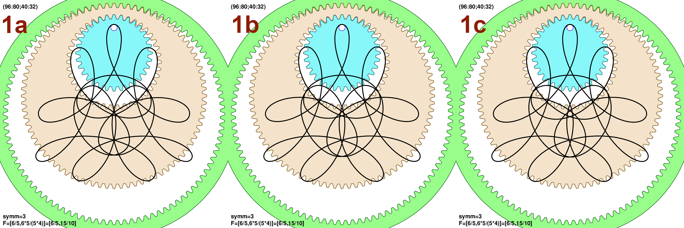
For the plot examples shown here I add a small circle on top of (Eq.2) to mimic the effect of the pen motion within the hole. The hole is about 2-3mm, or even larger, and there is small but appreciable motion of the pen inside it. This is popularly called “parallel lines” in the spirograph community as by inserting differently sized pegs one can obtain parallel lines on paper. I also rotate curves by \(90^\circ\) as it is easier to spot reflection symmetries. In most examples I use the 3rd, numerical, \(t_2(t_1)\) function as I am guessing that it is the closest to the pen trace on paper.
2 Comparison to wild gears on paper
I prepared a video with the gears in motion for two more accurate \(t_2(t_1)\) solutions. Youtube description contains links to videos with pen on paper using wild gears. At this moment I am not sure which of the two solutions is really the closest. We would need more precise parameters \(h\) and \(p\) to try to settle the question.
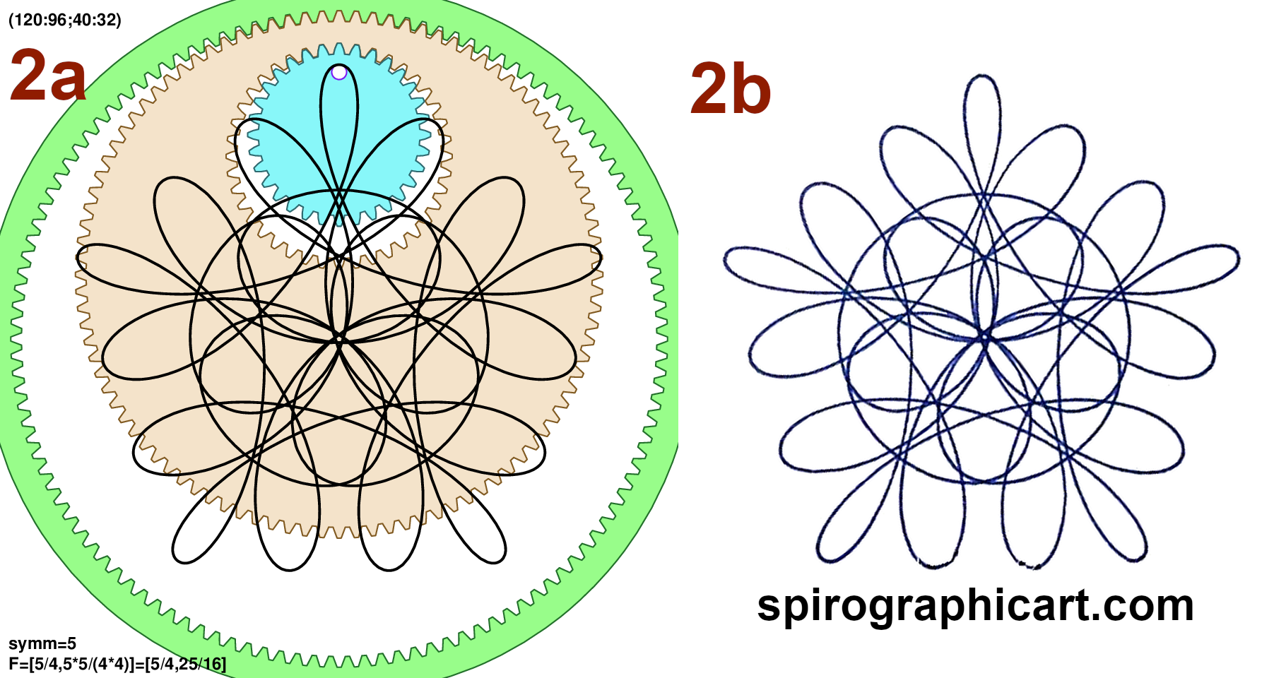
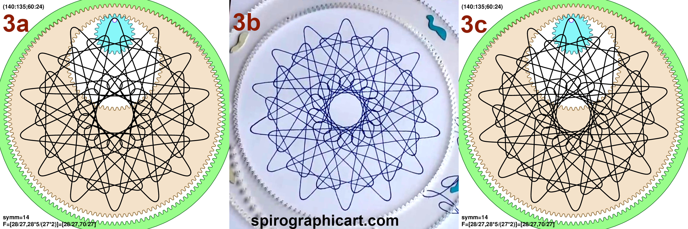
Figs 2 and 3 show comparison to two nice examples from spirographicart.com (many thanks!). Fig.2 is very good match. Fig.3a has correct outline, but is more symmetric compared to wild gears on paper in Fig.3b. However closely inspecting the setup with wild gears it seems that the smallest gear \(n_3=24\) doesn’t have pen-hole perfectly lined up. So instead of \(\varphi_p=0\) as in Fig.3a, trying half of tooth angular offset \(\varphi_p=\pi/n_3\) in Fig.3c makes a very good match. I think that this is a question of whether the pen-holes in gears align with the tooth center or with the gap, as wild gears come in both versions.
3 Two special cases and \(f_0\) and \(f_1\)
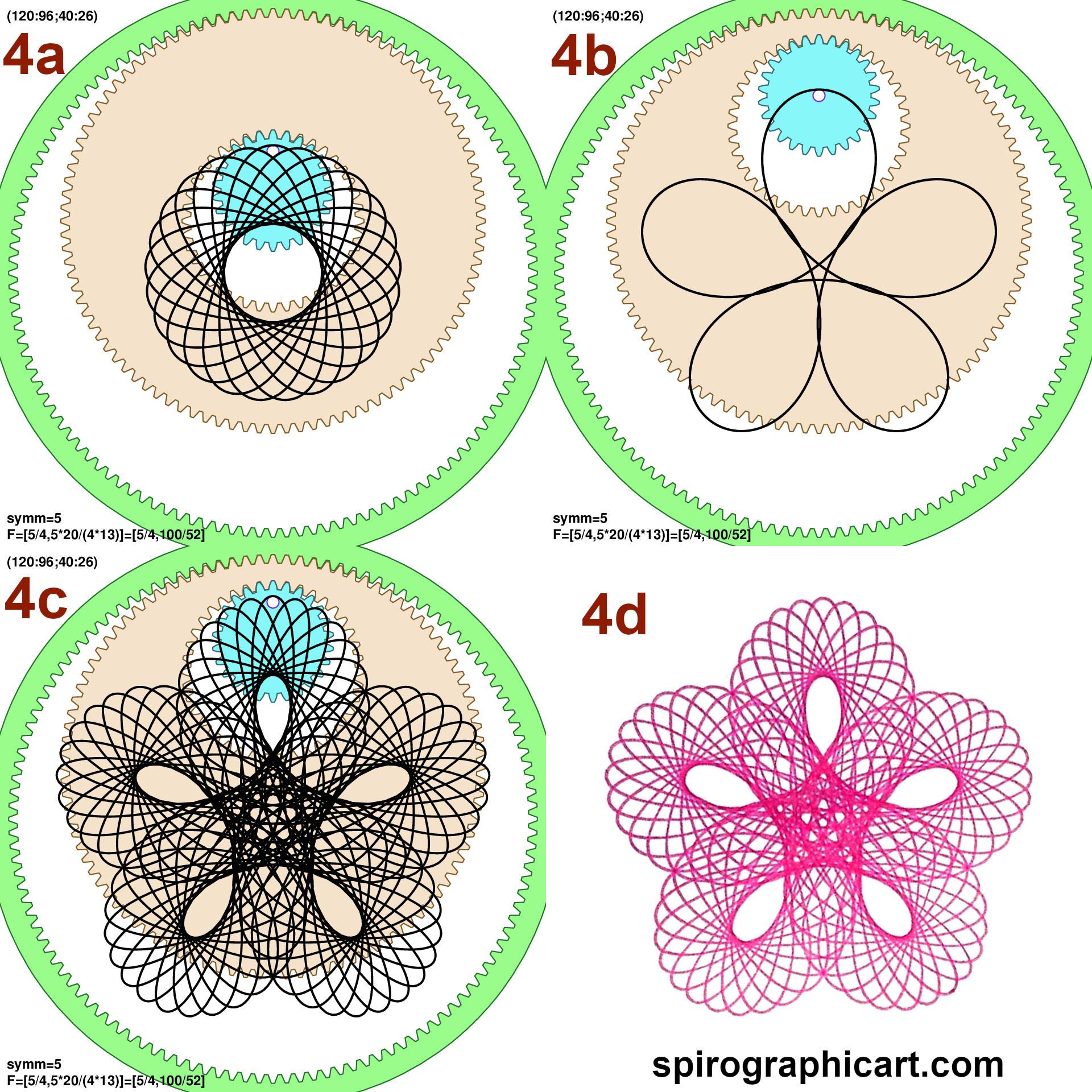
It is interesting to consider two special cases of the setup when the parametric equation simplifies. First case is when we have the middle “hoop” made of two concentric rings: \(h=0\) (but \(p>0\)). From (Eq.3.2) we obtain \(t_2=t_1\), and (Eq.2) reduces to only two simple harmonic terms \(x = A_1 * {\rm cos}(t) + B_1 * {\rm cos}(t-f_1 t)\) and \(y\) with sin() instead of cos(). We use \(f_1=n_0n_2/(n_1n_3)\) to denote ratio of numbers. The expression is functionally the same as ordinary spirograph, or the hypotrochoid parametric curve (Eq.1), except for different frequency \(f_1\). This setup was named “3) The Ring-Gear-Hoop system” by Aaron Bleackley where he used nomenclature that “hoop” denotes only the concentric rings case \(h=0\). Example of it is shown in Fig.4a. It is a simple figure, as \(f_1=120*40/(96*26)\) which simplyfies to \(f_1=25/13\): we have 25 simple lobes, and line connects every 13-th lobe.
Another simplification is obtained when we use a centered pen-hole in ring \(n_3\), or \(p=0\) (but \(h>0\)). With \(t_2=t_1\) the parametric equation (Eq.2) reduces again to only two simple harmonic terms \(x = A_0 * {\rm cos}(t) + B_0 * {\rm cos}(t-f_0 t)\), and \(f_0=n_0/n_1\). This is directly hypotrochoid parametric curve in (Eq.1). Example is shown in Fig.4b. Frequency is \(f_0=120/96=5/4\), thus we have 5 simple lobes.
4 General case
The general result for \(h>0\) and \(p>0\) in Fig.4c is just a simple modulation of Fig.4a on top of Fig.4b. For the gear combination (120:96;40:26) in Fig.4 it is particularly easy to “see” the modulation played out in our mind. Interplay of two frequencies or ratios is the most important aspect of the general case that it is worth repeating:
\[f_0 = \frac{n_0}{n_1} \tag{Eq.4.1}\] \[f_1 = \frac{n_0n_2}{n_1n_3} \tag{Eq.4.2}\]Both frequencies \(F=(f_0,f_1)\) determine the resulting curve. One of the most usefull quantities is: The number of times \(T\) that we have to turn inside the big stationary \(n_0\) wheel. We can notice that \(t=T*2\pi\) has to produce same value of sine and cosine terms in (Eq.2) as \(t=0\). Or \({\rm cos}( f_0t )\), \({\rm cos}( f_1t )\), and same with sine terms. This is only possible if \(f_0T\) and \(f_1T\) are integers. In other words \(T\) is least common multiple (lcm) of \(f_0\) and \(f_1\) denominators. In turn denominators of irreducible fractions \(f_0\) and \(f_1\) can be written using greatest common divisors (gcd)
\[T = {\rm lcm}\bigl( {n_1}/{ {\rm gcd}(n_0,n_1) }, {n_1n_3}/{ {\rm gcd}(n_0n_2,n_1n_3) } \bigr) \tag{Eq.5.1}\]The above expression is the easiest way to calculate \(T\) by hand. But after comparing with the Alyx Brett work I realized that after some lcm/gcd algebra it could be written in a perhaps neater looking form as:
\[T = \frac{1}{n_0n_2} {\rm lcm}\bigl( n_0n_2,n_1n_2,n_1n_3 \bigr) \tag{Eq.5.2}\]Implementing above equation requires usage of 64 bit integers as it can overflow.
If \(T\) is large, which is typically the case unless teeth numbers are a bit commensurable, the result might be tearing the paper. For example (120:96;40:26) in Fig.4 we have \(f_0=5/4\) and \(f_1=25/13\), thus \(T =13*4\) indicating heavier drawing. In contrast in Fig.1 we have \(F=(6/5,3/2)\) and thus \(T = 2*5\), indicating a light curve. Number of rotations of \((n_1;n_2)\) hoop is
\[T_1=f_0*T \tag{Eq.6.1}\]while the number of rotations of the innermost gear \(n_3\) is
\[T_3 = f_1 * T \tag{Eq.6.2}\]And a very usefull connection:
\[F=(T_1/T,T_3/T) \tag{Eq.6.3}\]Or: despite strange looking equations we are just putting two fractions into a simplest form with a common denominator. In my plots I express \(f_1\) with the common denominator to \(f_0\) and then it simply reads \(f_1=T_3/T\). Similarly to ordinary spirograph, the numerator \(T_3\) is also the number of lobes in the curve, though this can be hard to see in busy figures.
5 Rotational symmetry
One way to obtain rotational symmetry is to again examine sine and cosine arguments of (Eq.2) and ask when is the result unchanged under rotation. But a simpler deduction could be made from the observation that the final curve is modulation of hypotrochoid \(f_1\) on top of the base hypotrochoid \(f_0\) (cf. Fig.4). The total symmetry has to be symmetry of both. When \(f_0\) and \(f_1\) are expressed as irreducible fractions their respective rotational symmetries are given as numerators. Thus the total symmetry is greatest common divisor (gcd) of those 2 numerators. This is simpler to express using number of rotations \(T_1\) and \(T_3\) from above:
\[n_{\rm symm} = {\rm gcd}( T_1, T_3 ) \tag{Eq.7}\]Rotation by \(2\pi/n_{\rm symm}\) will leave curve unchanged. Note that the curves always have \(n_{\rm symm}\) rotational symmetry, regardless of the initial condition \(\varphi_p\). I didn’t work out comparison to Alyx Brett results on rotations, but I think they are the same.
Plugging actual numbers for typical wild gear elements we mostly get low symmetry, or none at all \(n_{\rm symm}=1\). The teeth numbers should be a bit commensurable to get symmetric outcome. Two nice curves with higher rotational symmetry are shown in Fig.5.
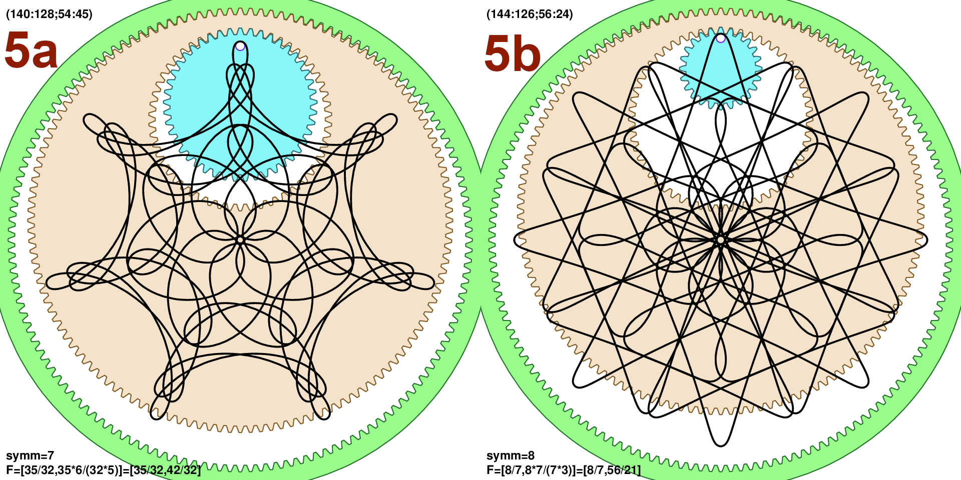
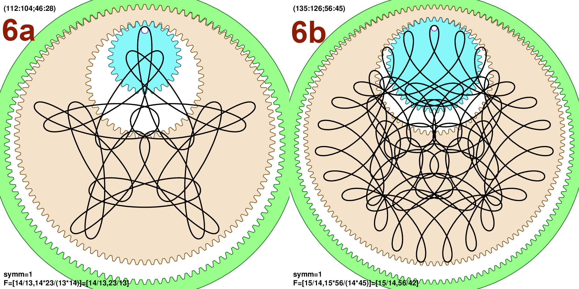
But there is also a fun category of curves that on the first glance look like they posses rotational symmetry, but not really at details level as their \(n_{\rm symm}=1\): Fig.6.
6 Reflection symmetry
In contrast to rotational symmetry curves only sometimes possess reflection symmetry, depending on the initial condition \(\varphi_p\). To work this out we notice that for a curve to have reflection symmetry the smallest gear \(n_3\) has to be aligned with the \((n_1;n_2)\) hoop at some point \(t\) during the trajectory. Meaning that at some point both \(t_2\) and \(t_3+\varphi_p\) should be multiples of \(\pi\). After some algebra we obtain that for the reflection symmetry the initial pitch of the innermost cog \(n_3\) has to be
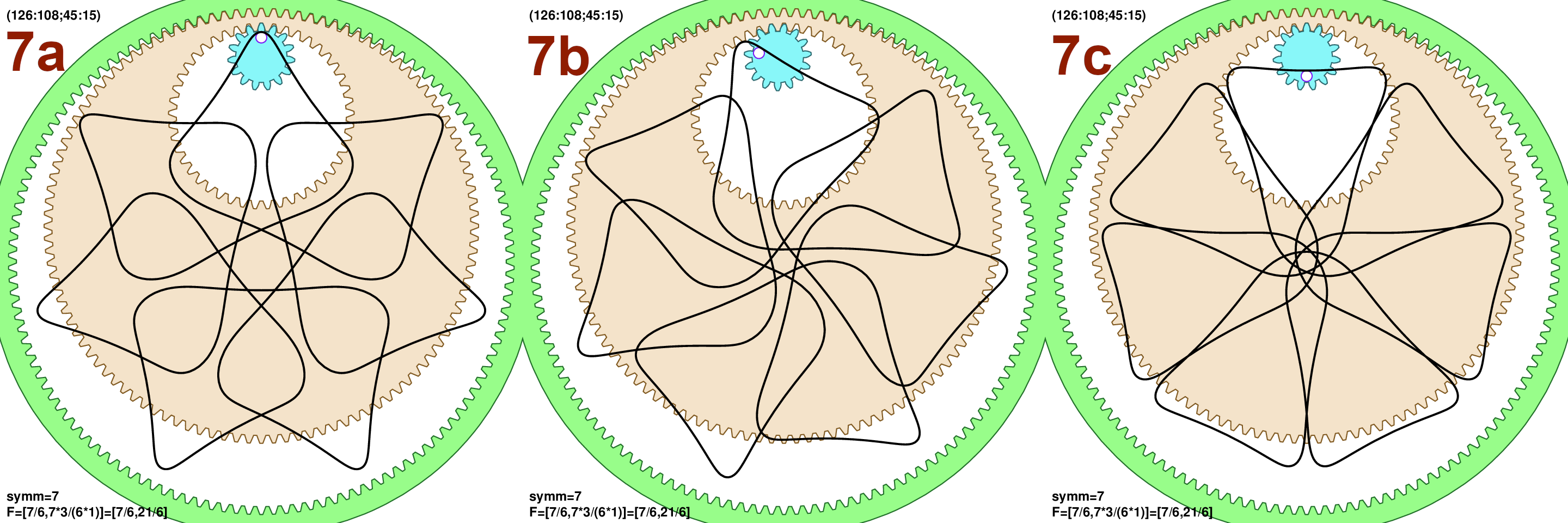
\[\varphi_p = k*\pi n_{\rm symm}/T_1, k \in \mathbb Z \tag{Eq.8}\]The next result I didn’t formally prove: the set of pitch values \(\varphi_p\) from (Eq.8) produces only two distinct curves, one for even and one for odd integers \(k\). Reflection axis itself may be rotated though, but the curves are the same. This also means that \(\varphi_p=0\) and \(\varphi_p=\pi\) can produce the same curve, depending on whether \(T_1/n_{\rm symm}\) is even or odd. (Eq.8) is also useful as it suggest \(k=1/2\) as a choice for curves that have most slant and visual deviation from reflection symmetry. In Fig.7 we show \(k=0\), \(1/2\) and \(1\). Fig.7b is slanted and doesn’t have reflection symmetry.
7 Simple numerical example
Lets work out a simple numerical example by hand. Consider gear system (126:108;45:15) from Fig.7. Frequencies are \(f_0=126/108\) and \(f_1=(126*45)/(108*15)\). To reduce the fractions we keep trying to divide out small factors. Or, if this is made by wild gears there are probably prime factors written on gears. For \(f_0\) we divide out \(2*3^2\) and obtain \(f_0=7/6\). For \(f_1\) we divide out \(2*3^4*5\) and get \(f_1=7/2\). Then two fractions \(7/6\) and \(7/2\) should be brought to the same denominator: \(7/2=21/6\). Thus \(F=(7/6,21/6)\) and we read: \(T_1=7\), \(T_3=21\) (curve has 21 “lobes”), and \(T=6\) meaning that it is a light curve as we turn only 6 times inside the stationary ring. The rotation symmetry is the least common denominator of fraction numerators: common of \(7\) and \(21\) is \(n_{\rm symm}=7\), so it is a 7-fold symmetric figure.
8 Inversion from frequencies
One very useful method is to start from given frequencies \(F=(T_1/T,T_3/T)\) and then find teeth numbers for all 3 elements \((n_0:n_1;n_2:n_3)\). It is a better approach for exploration as the frequencies directly control curve properties. We need to assume that numbers \(T_1\), \(T_3\) and \(T\) don’t have a common divisor (if they have we can just divide that out). Cogs should also fit into the outer cogs: \(T<T_1<T_3\). Next we need number of rotation symmetries \(n_{\rm symm}={\rm gcd}(T_1,T_3)\) and a parameter \(n_h={\rm gcd}(T_1,T)\). Simple rearrangement of the equations from Section 4 yields \(n_0=a*T_1/n_h\), \(n_1=a*T/n_h\), \(n_2=b*T_3/n_{\rm symm}\) and \(n_3=b*T_1/n_{\rm symm}\), where \(a\) and \(b\) are arbitrary positive integers. Well, we still need physically possible system so number of teeth should differ by at least 6 - 8. Also \(n_1\) and \(n_2\) should be sufficiently different to allow larger hoop offsets \(h\). Small \(h\) tend to be look bland. Maximal possible value for \(h\) is such that \(n_1\) and \(n_2\) touch: \(h_{\rm max}=1-n_2/n_1\). But just increasing \(a\) is sufficient: \(h\) values of 0.4 - 0.6 look interesting enough.
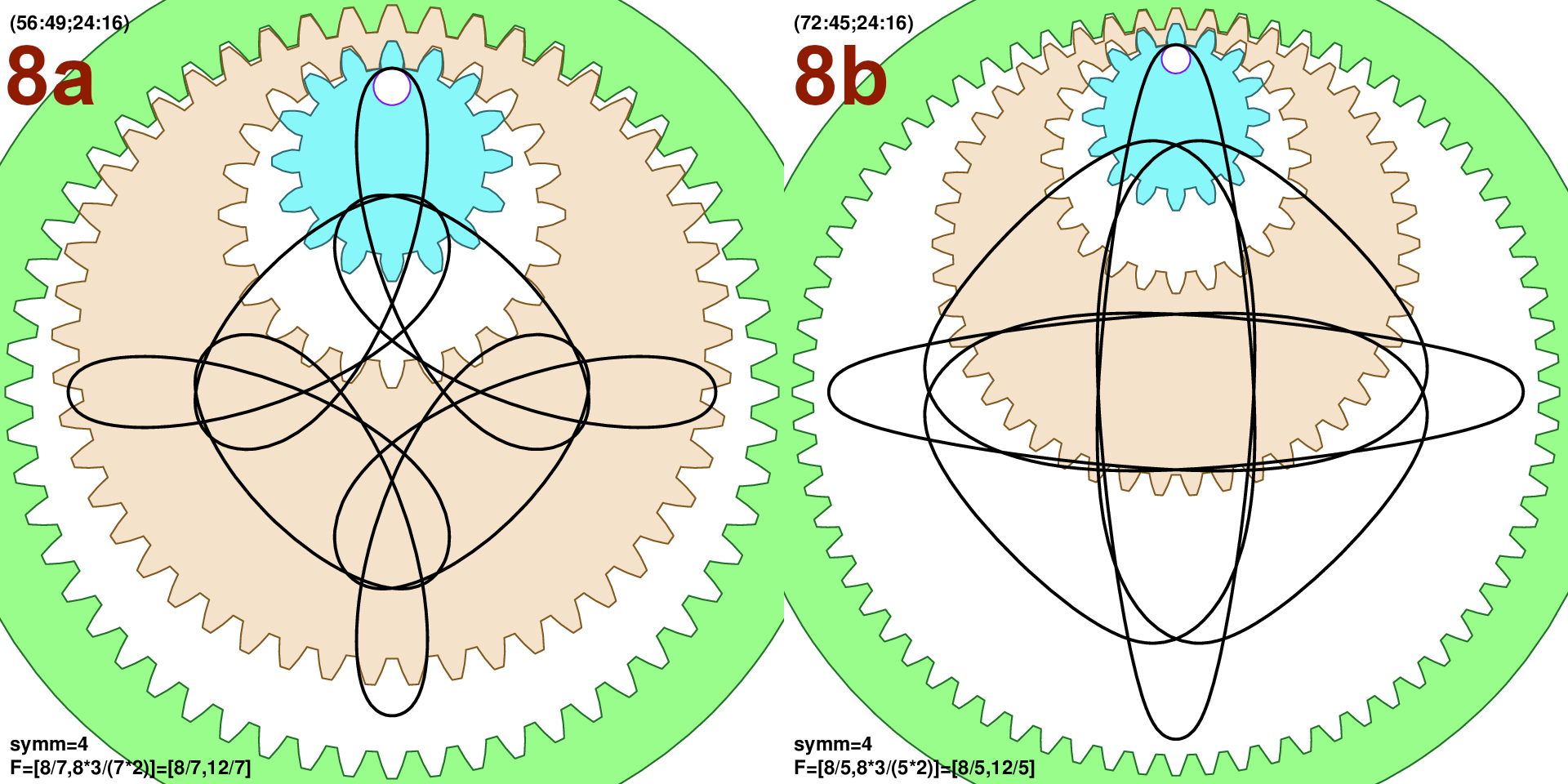
Example 1: Frequencies \((16/14,24/14)\) are not reduced, as we can divide further all 3 numbers with 2. Thus starting point can be \(F=(8/7,12/7)\), or \(T_1=8\), \(T_3=12\) and \(T=7\). Then number of rotation symmetries is \(n_{\rm symm}={\rm gcd}(8,12)=4\). This will be a light curve (\(T=7\)) with 4-fold symmetry. It will have \(T_3=12\) lobes. Parameter \(n_h={\rm gcd}(8,7)=1\). Out cog system is \(n_0=8a\), \(n_1=7a\), \(n_2=3b\) and \(n_3=2b\). Some minimal numbers so that wheels differ by at least 7 teeth are \(b=8\) and \(a=7\) or (56:49;24:16).
Example 2: Lets try something similar \(F=(8/5,12/5)\). Again: \(n_{\rm symm}=4\) and \(n_h=1\), and this is even a lighter curve (\(T=5\)). The cog system is \((8a:5a;3b:2b)\). Try \(b=8\) and \(a=9\) and we get (72:45;24:16). Fig.8 shows our two examples. It also demonstrates that number of teeth need not be very large. Since \(a\) and \(b\) are arbitrary there are many possible ways to archive any pair of F-ratios.
9 Gallery of curves and online plotter
The second order roulette produces truly wild curves. This is by far the most interesting extension of the ordinary spirograph. I prepared a slide-show of interesting curves on youtube. My method was to pick parameters from “more common” gears and hoops from basic wild gears collections, generate couple of thousand curves and their properties and then automatically sub-select for lighter curves (smallish \(T\) and/or not too big \(T_3/T\) and/or higher symmetries). The shown curves should all be possible to draw with pen on paper with wild gears. I also tried to note when different cog combination produces the same frequencies since that will generate a similar curve.
I also wrote a basic plotter in javascript: here. The tool uses (Eq.2) and (Eq.3.2) and can visualize curves. It might not be super stable (just reload the page in different tab). The tool can also invert frequencies (scroll down) and this is probably more interesting application.
10 Gear on gear or weird shapes and such
All equations so far are valid even for some negative \(n\)-numbers, or for inversion \(n_0<n_1<n_2<n_3\). These are meaningful combinations that describe gear in hoop mounted on the outside of a fixed gear, or wheel rotating around hoop around fixed gear and such. In the above expressions one occasionally needs absolute value, but equations are still valid. It is also interesting to see weird shapes such as triangles or squares, rotating. All those are second order roulettes. I will try to prepare some material in the future, as this is already a very big article.
11 Third order roulette
How about a third order system, with one more hoop inserted \((n_0:n_1;n_2:n_3;n_4:n_5)\)? As demonstrated by a reddit user it does seem possible. Parametric description is not much harder than illustrated above for the 2nd order: it is straightforward to extend (Eq.2) with one more block. Fundamental ratios or frequencies are
\[f_0 = \frac{n_0}{n_1} \tag{Eq.9.1}\] \[f_1 = \frac{n_0n_2}{n_1n_3} \tag{Eq.9.2}\] \[f_2 = \frac{n_0n_2n_4}{n_1n_3n_5} \tag{Eq.9.3}\]The task is again to bring fractions to a common denominator \(T\): \(F=(T_1/T,T_3/T,T_5/T)\). The number of rotations within static ring \(n_0\) is \(T\), while there are \(T_5\) “lobes” in total. Though what counts as a “lobe” is even more stretched, basically most kinks count. And as above for the 2nd order, the number of rotation symmetries is \(n_{\rm symm}={\rm gcd}(T_1,T_3,T_5)\). Here are two examples:
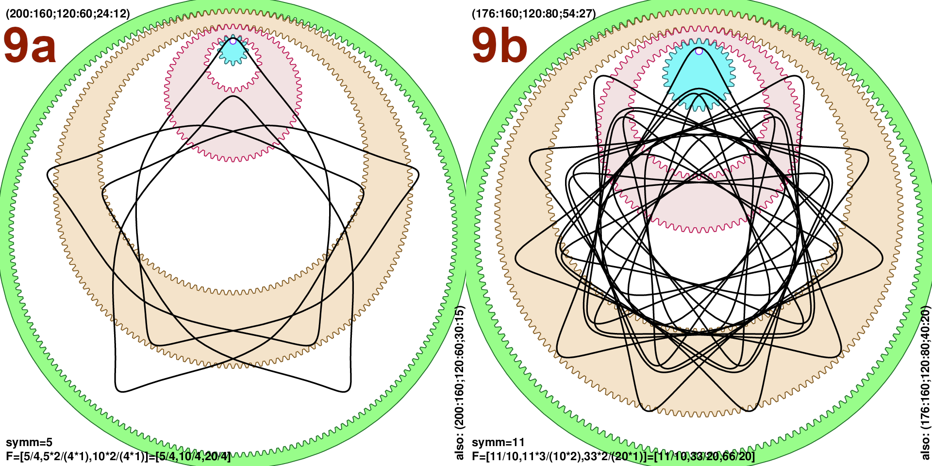
Let us work out numbers for Fig.9a: from (200:160;120:60;24:12) we have \(f_0=200/160=5/4\), \(f_1=200*120/(160*60)=5/2\) and \(f_2=200*120*24/(160*60*12)=5\). The 3 fractions should be brought to same denominator: \(F=(5/4,10/4,20/4)\). We read \(T=4\) and \(T_5=20\), while symmetry \(n_{\rm symm}={\gcd}(5,10,20)=5\), i.e. very light figure with 5-fold symmetry.
The actual problem with 3rd order roulette is that most of the time the number of rotations \(T\) within the static ring \(n_0\) is huge! My first attempt at creating a gallery of examples was pittifull, as most combinations produced \(T\) close to 1000 or more. Good only for ripping the paper. Therefore I expanded my set of hoop parameters and got some 100 moderate examples shown in this youtube slide-show. Downside is that the examples are probably not easy to reproduce as they contain hoops from less popular sets.
In the end I have to admit that I don’t have wild gears (I will get something…) and this section on 3rd order curves is least checked. There are many online examples of the 2nd order roulette and I consider it well checked. For the 3rd order I can match that single example from reddit, but it is unfortunate as it is of lower complexity since the first hoop was concentric \(h_0=0\). Please let me know if you produce some examples on paper, I am very interested to compare the curves. I sugest then to try to perfectly line up 2 hoops and the pen-hole, as sometimes it is very hard to guess such offset parameters.
12 Post-publication notes
Here are some notes that came after the original publication.