Grid of roulettes
Lets further explore the weird world of the 2nd order roulette curves. Or gear-in-hoop-in-wheel spirograph.
My previous slideshow of curves was aimed to be easier to reproduce with wild gears. I tried to limit the choice of cogs to basic wild gear sets. New slideshow video expands the cogs and shows more of the crazy curves, but it will probably be harder to reproduce on paper.
Another interesting approach is to make a grid of outcomes. Since there are 10-20 available non-concentric hoops there is a point to just keep adding different gears n3 and wheels n0 to the same hoop (n1;n2). This makes a nice grid of (n0:n1;n2:n3) curves.
The first on display is the hoop (72;36) from the most basic wild gears set (click on the image for large version):

To produce the image I run all combinations of gears and wheels and try to select for lighter curves (smaller T from the previous articles). But not all hoop grids make interesting images. Boring ones are (108;25), (104;46), or (128;38) as most of the outcomes are “a messed up black blob” or “ropy” like ordinary hypotrochoids. Clearly some commensurability is needed. But not too much, as for instance, (64;32) grid is not much varied either.
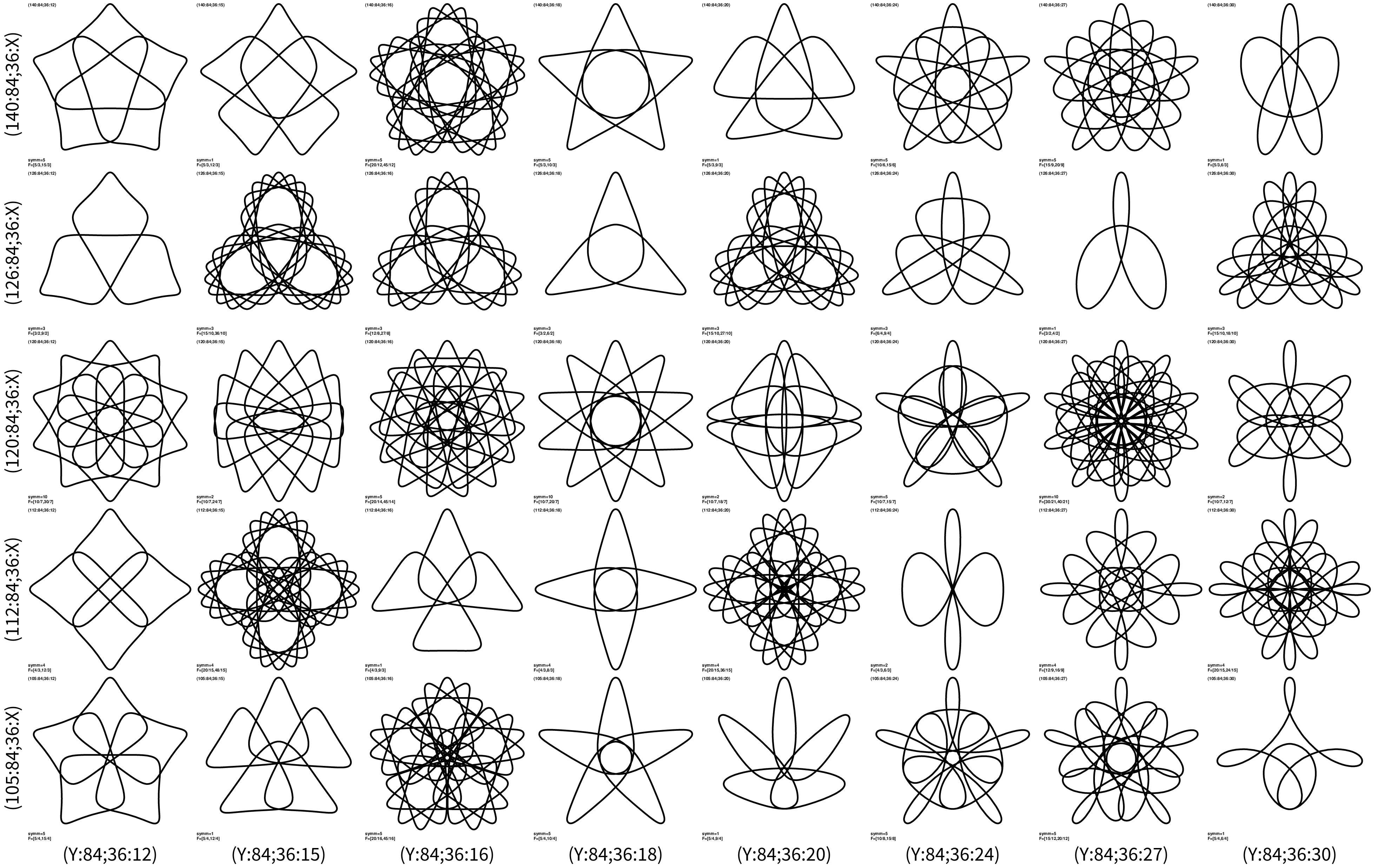
A few interesting grids. (84;36) hoop:
Or (105;40) hoop:

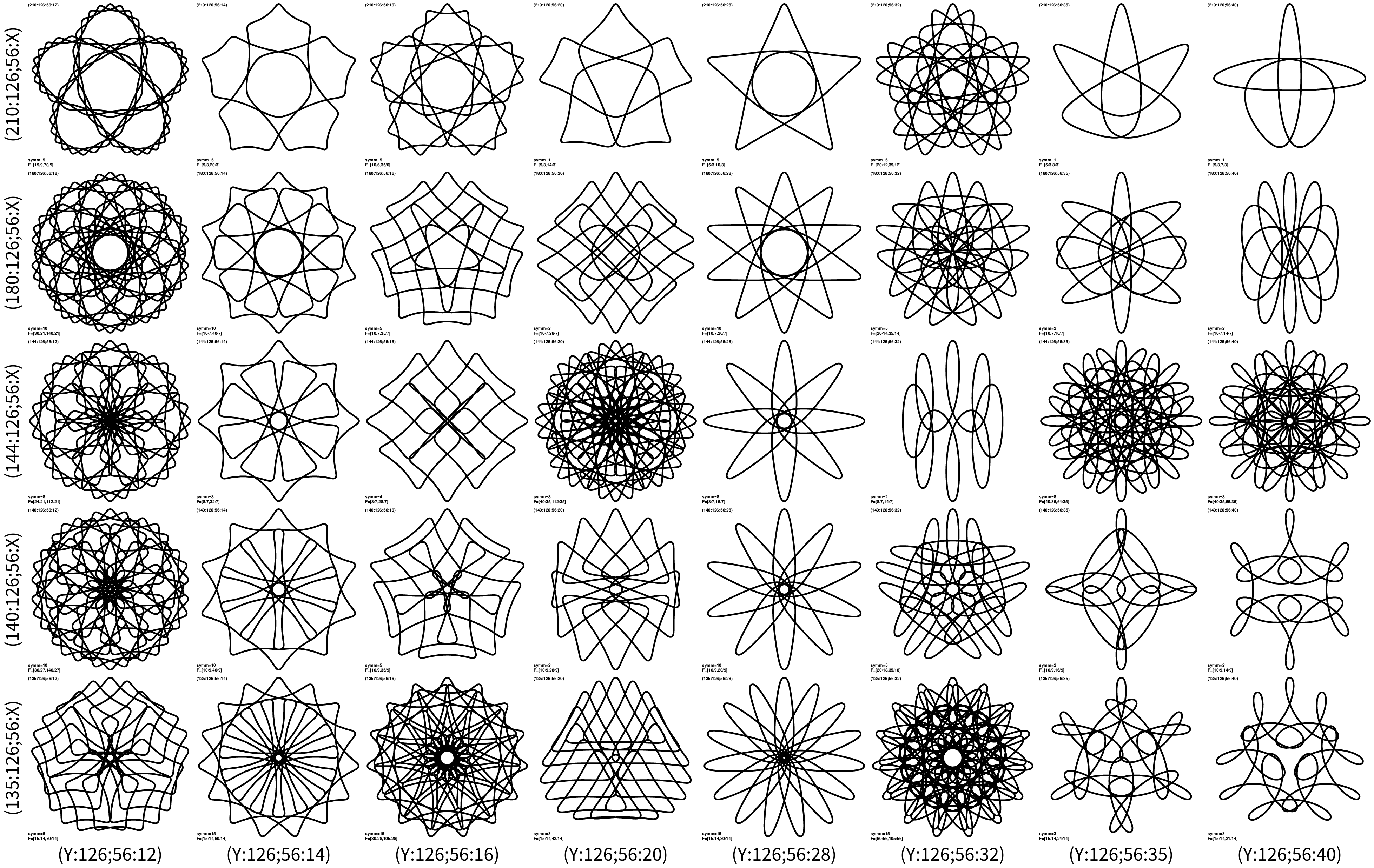
(126;56):
The selection criteria I used to organize grids seems to prefer more symmetric shapes to be displayed in this way. There are always a lot of asymmetric curves (nsymm=1) when I search through parameters, but they don’t end often on grids.