Survey of roulettes
The goal of this article is to try to systematically survey 2nd order roulette curves. Or gear-in-hoop-in-wheel spirograph. Three most important parameters are 3 numbers T, T1, and T3 that form ratios or frequencies F=(T1/T,T3/T). However that is one parameter too many for any systematic display, since 2D grids work best. At least for me. But it turns out that T is the least important parameter. For instance look at the expression for the number of rotational symmetries: nsymm=gcd(T1,T3), it does not contain T.
Since T is less important parameter we can make T1 vs T3 grid of curves. Though that still leaves a question of how to select a “representative” value of T. I have a few hundred “nice” looking curves in few galleries. That set has various parameters, but on average it seems that T is close to about 0.8T1 for most of the curves. Such a choice (pick an integer T close to 0.8T1) is a good choice, but I found one even better criterion: It comes from the observation that when the cogs are very different in size the outcome starts to be easy to predict, such as “ropy spirograph” pattern. Thus for a given T1 and T3 we can examine all possible values of T<T1 (inversion procedure) and select a value T that gives the smallest ratio of the wheel to gear size: n0/n3. Such a choice forces gears to be of similar size, as much as possible, and that in turns makes lines from different cog turns cross and mix more. That doesn’t mean it will always look the best, but to me it seems that more often than not it produces striking patterns.
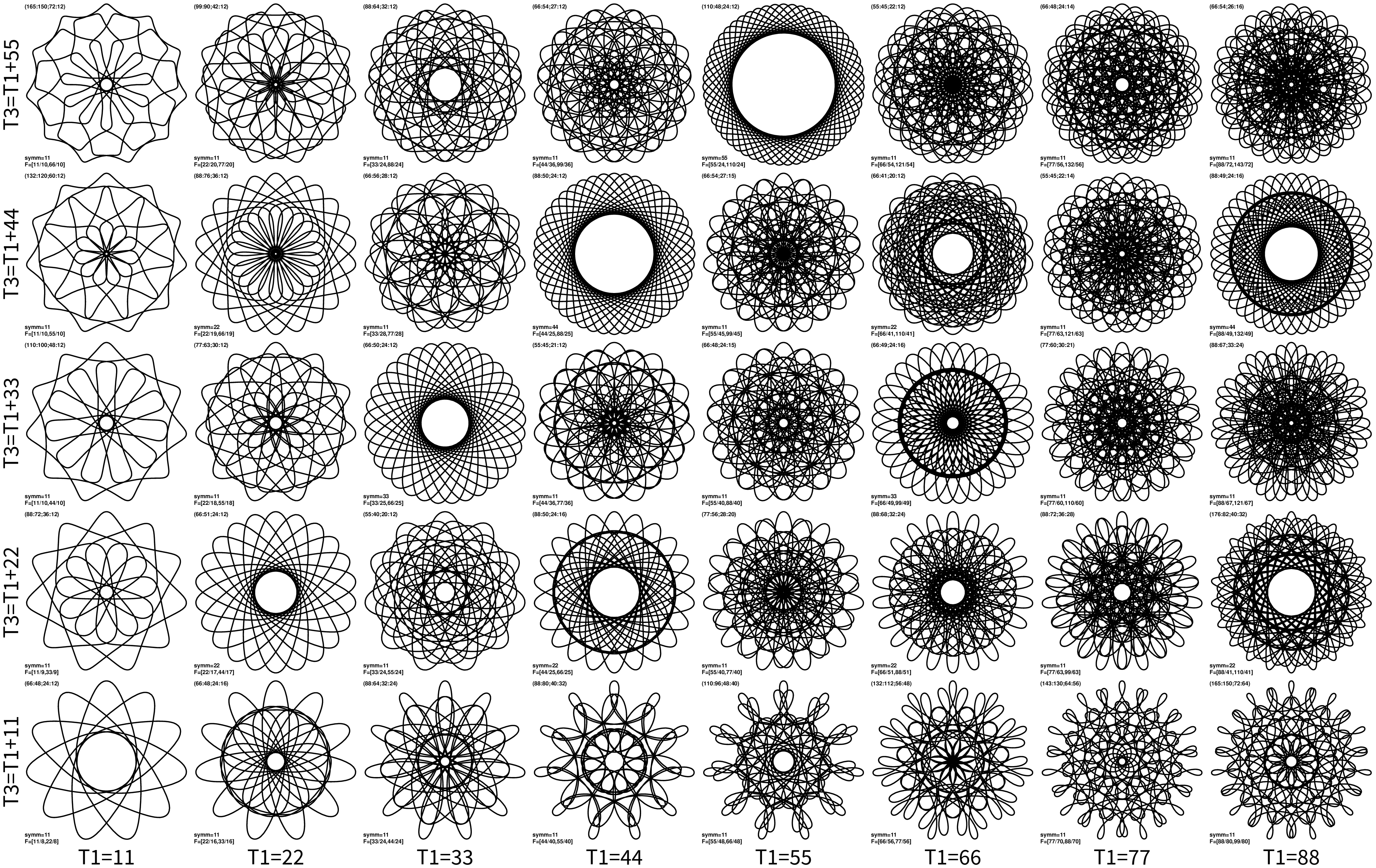
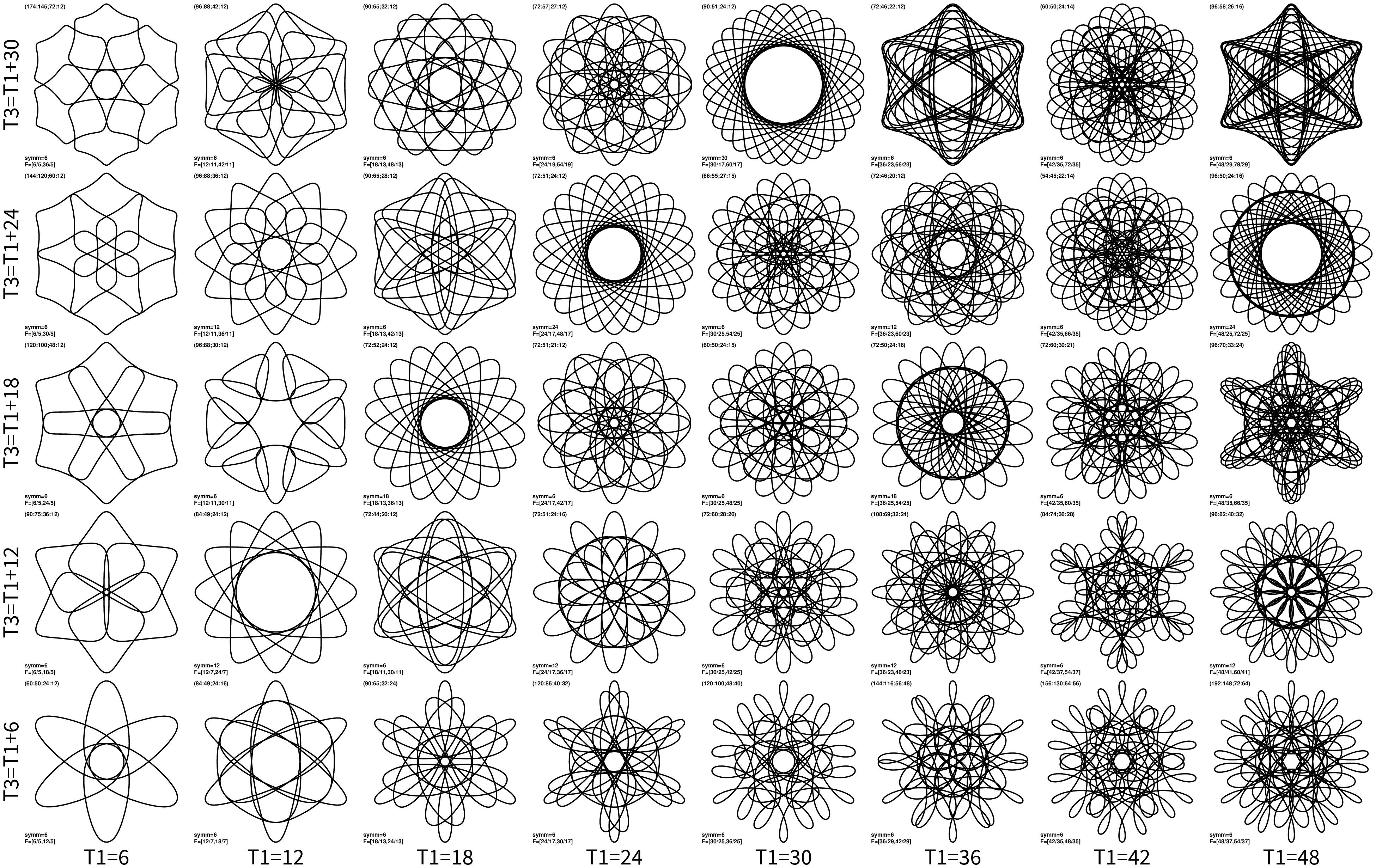
Finally we can produce 2D grids but aim for specific rotational symmetries, i.e. lets try to show for instance only nsymm=7 grid. Then the choice of X axis is T1=7x, where x is positive integer. Since we need to observe condition T1<T3 using T3=7y would make half of the plot empty. A more compact form is to use T3=T1+7y, where y is positive integer. This will give at least 7-fold symmetry, but in quarter of the cases it will make 14-fold symmetry (e.g. x=4 and y=2), and in 1/9 cases 21-fold, etc. I decided to keep those higher symmetries in the plot, as it looks better than leaving blank panel (click on the image for large version):
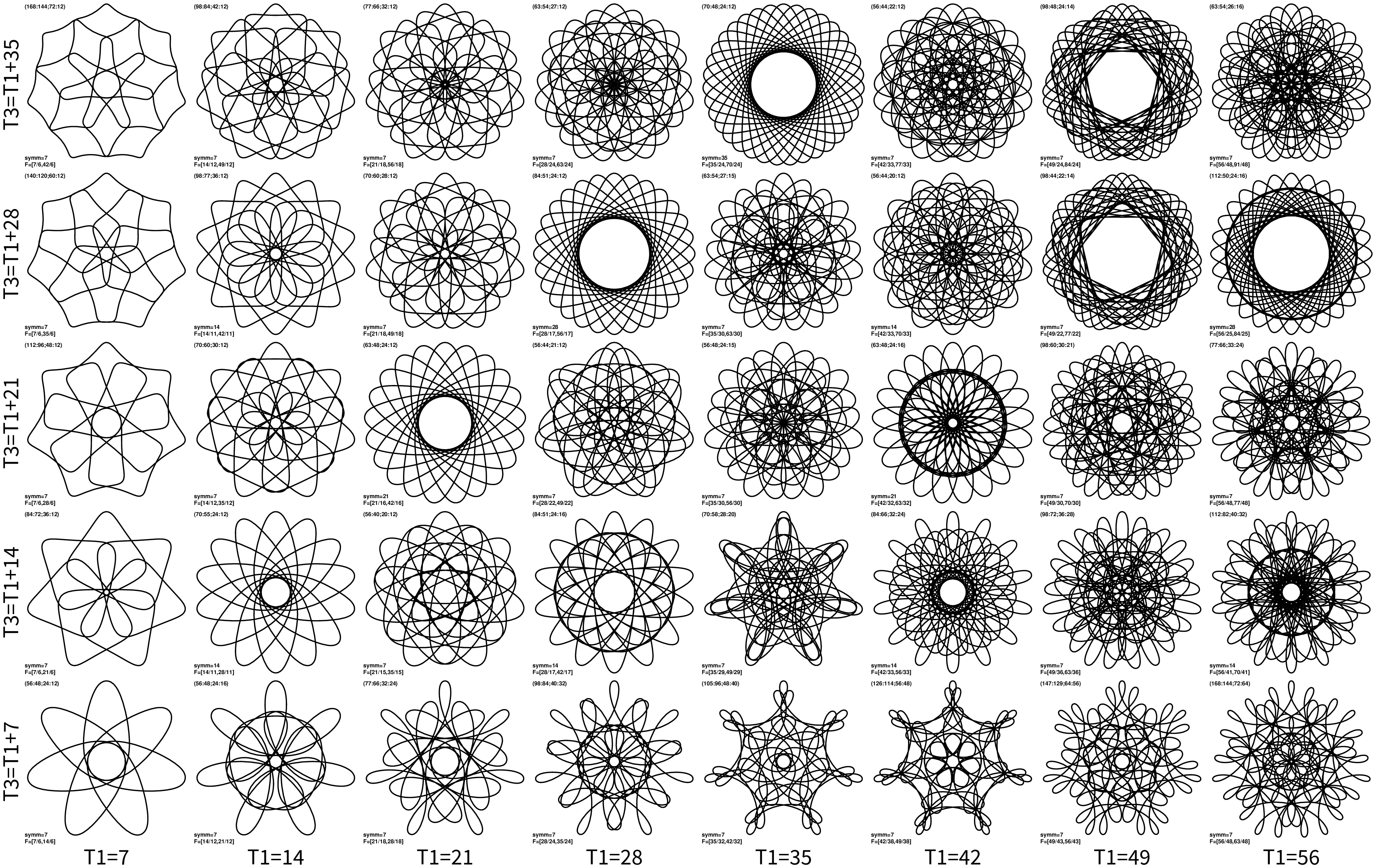
The image is really striking, and more ordered than naively expecting. I did expect, for instance, that diagonal x=y resembles ordinary spirographs, as that is just doubling the frequency (i.e. T3=2T1). But there are other patterns as well. One strongest is for instance along the line (x=2,y=1), (x=4,y=2), (6,3) and (8,4) shapes are also similar in a way: there are individual lobes sticking out of a disk pattern. This is also some beating of frequencies, as numbers can be summarized as 2T3=3T1. Patterns also separate in type. Lower-right has lobes sticking out, while the upper-left side is more disc or rose like.
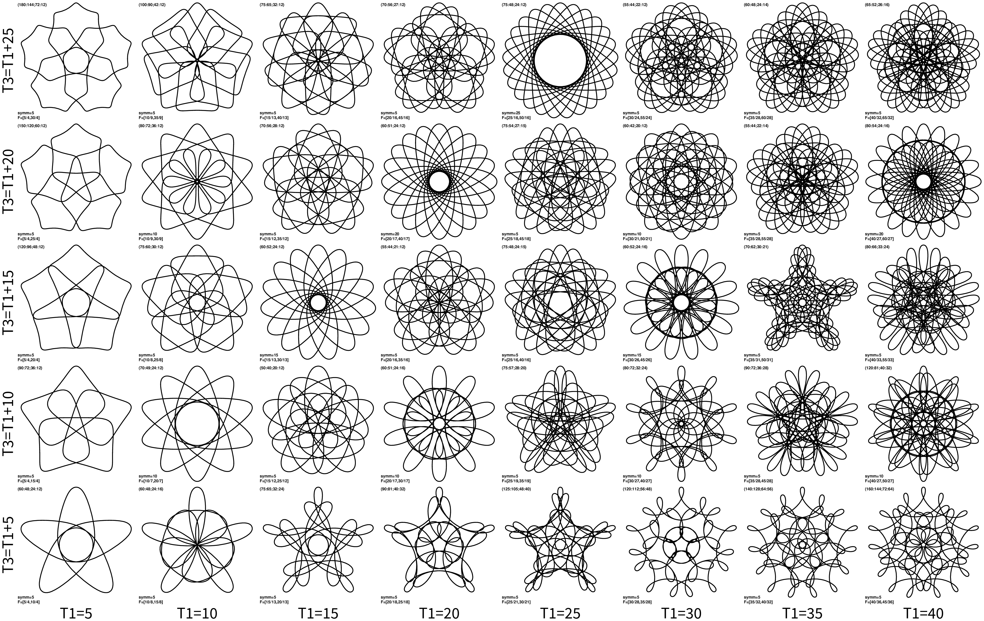
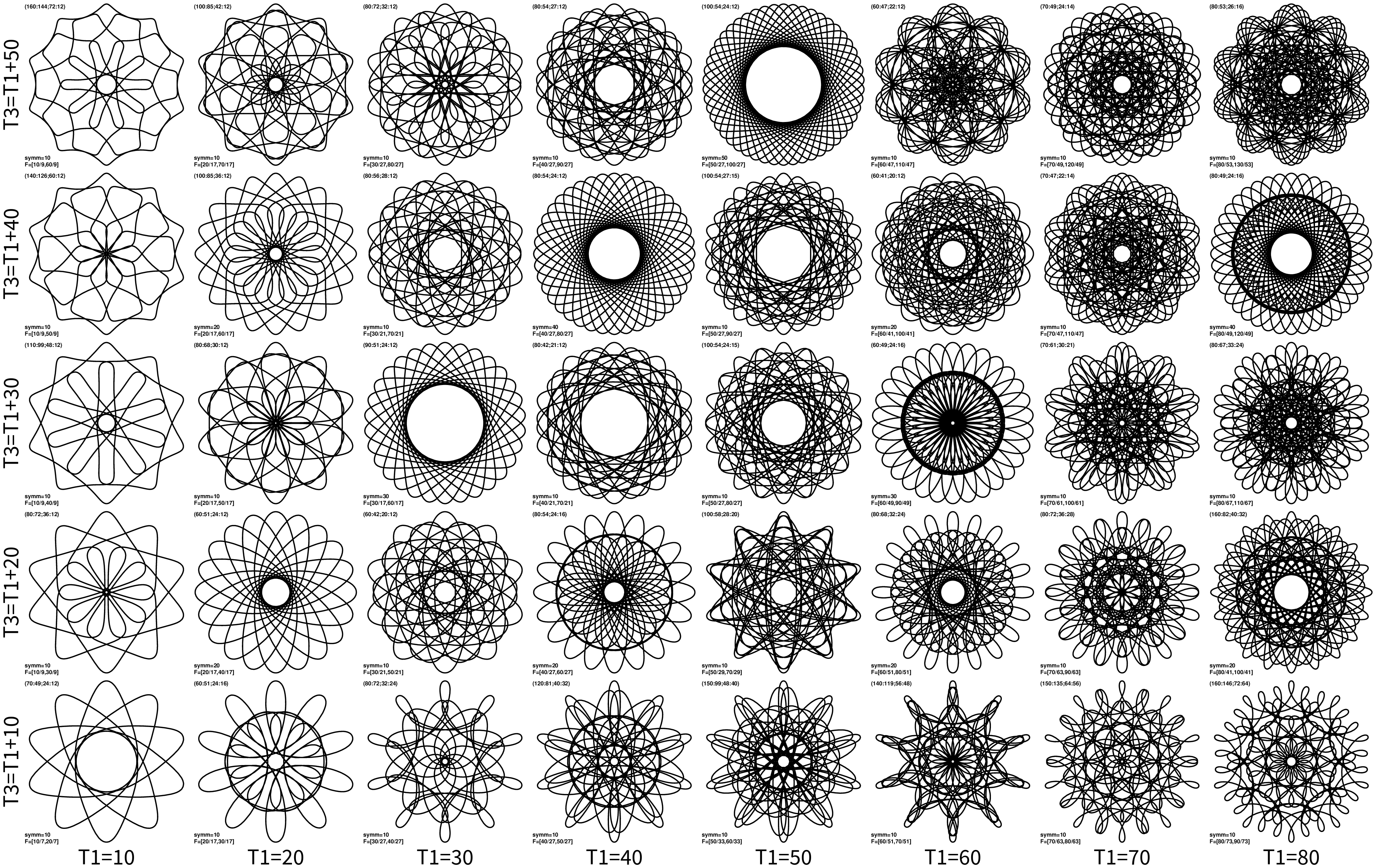
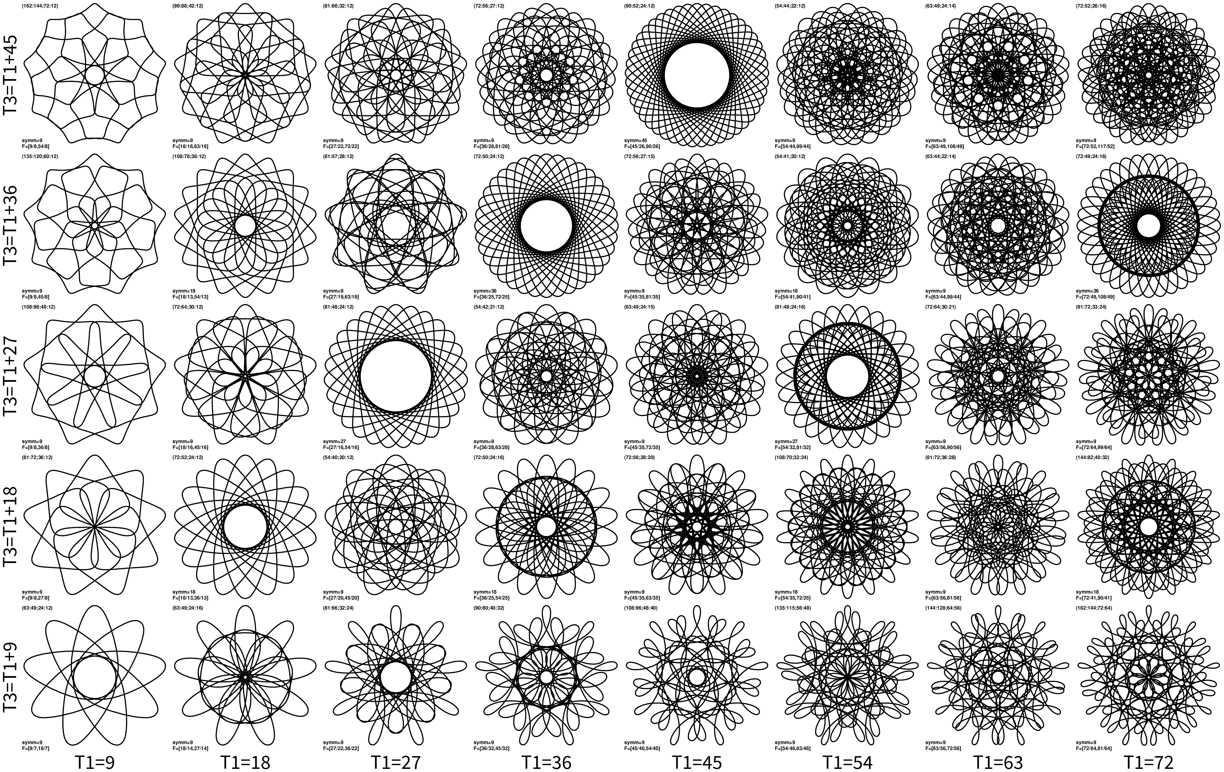
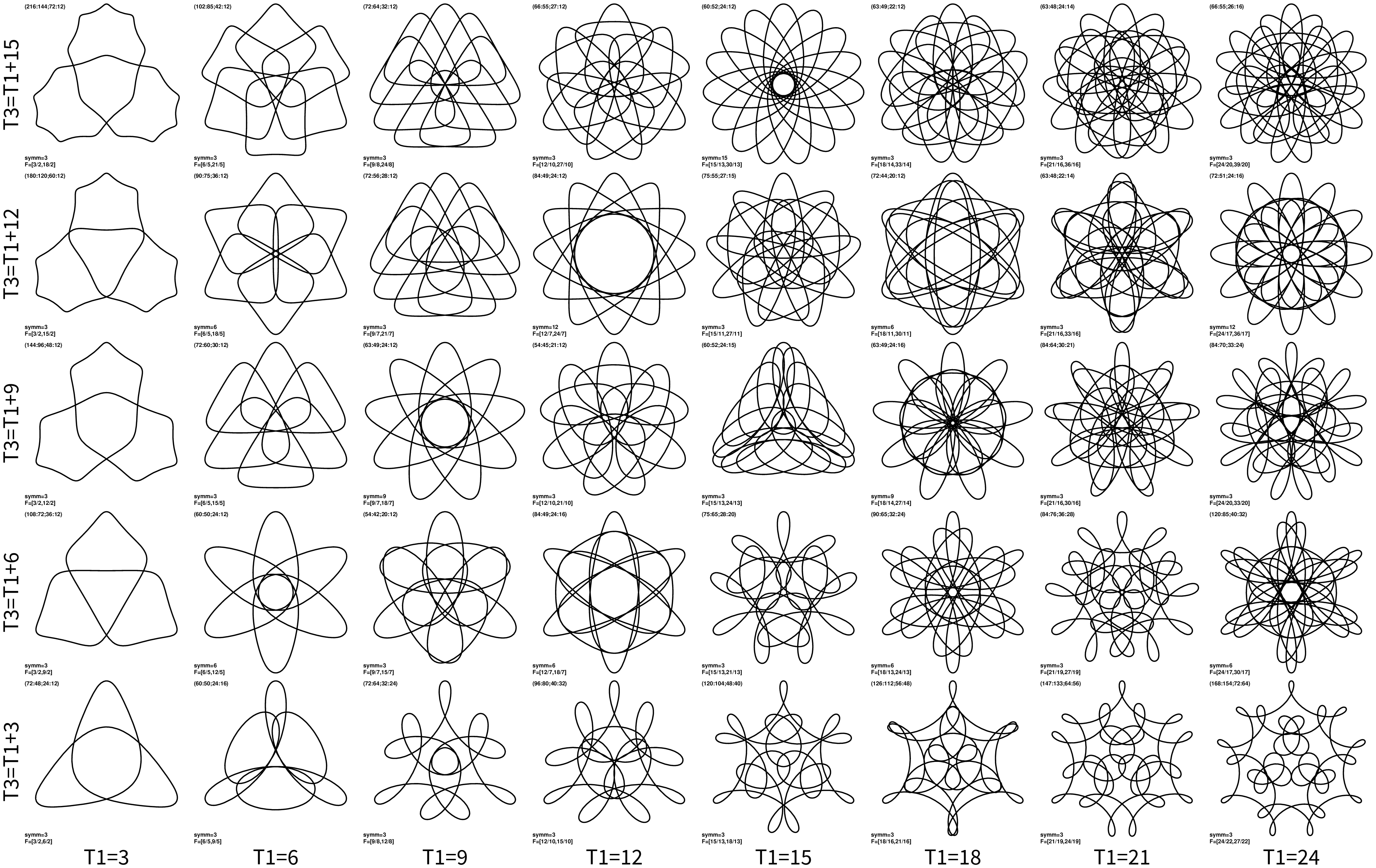
And interestingly there is a strong resemblance between individual panels to other nsymm values. For instance compare above plot to nsymm=5 grid:
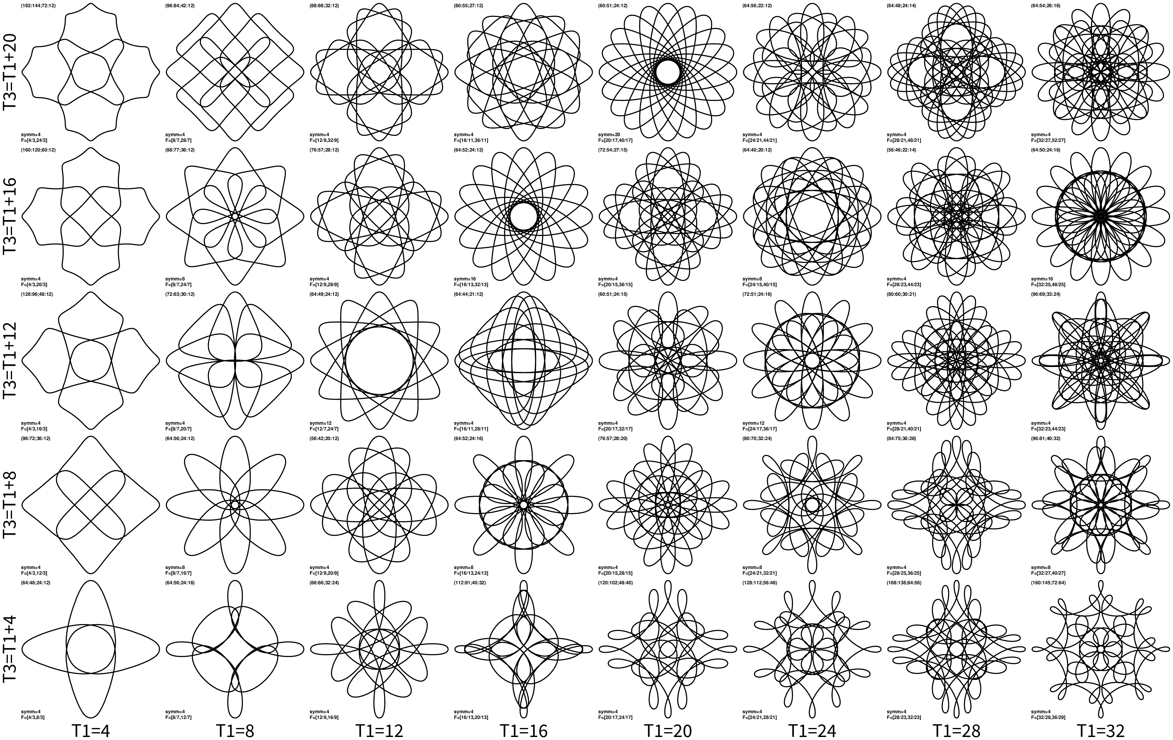
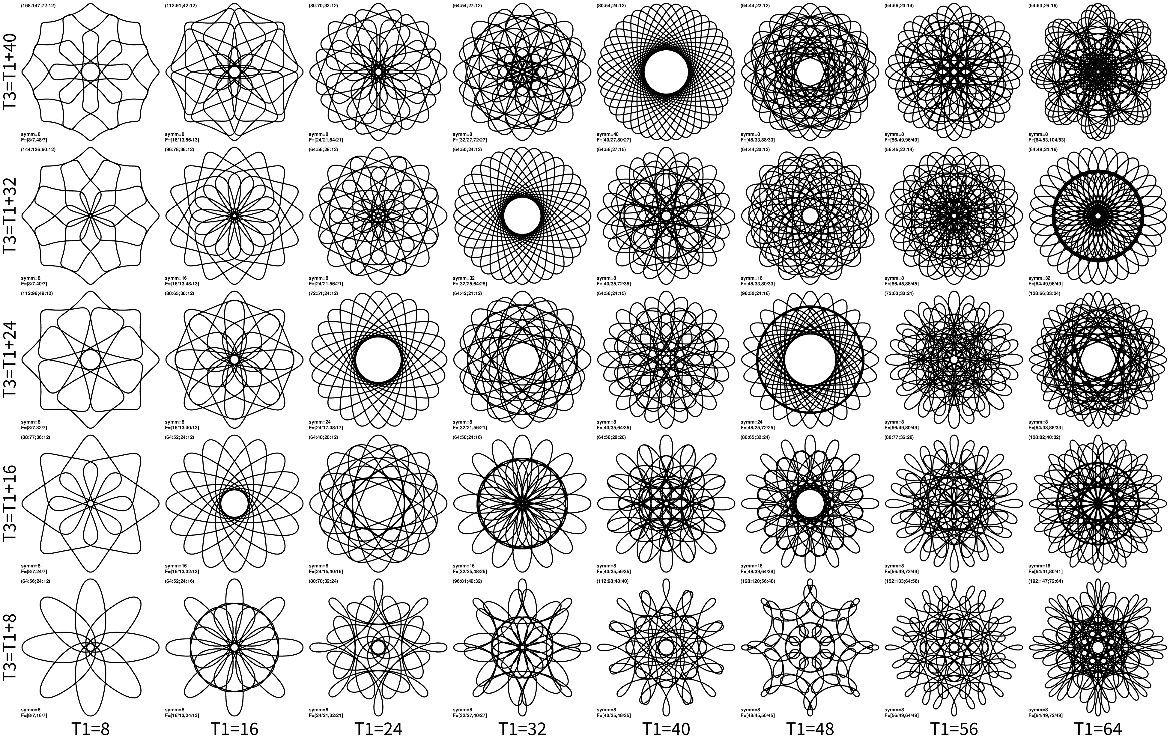
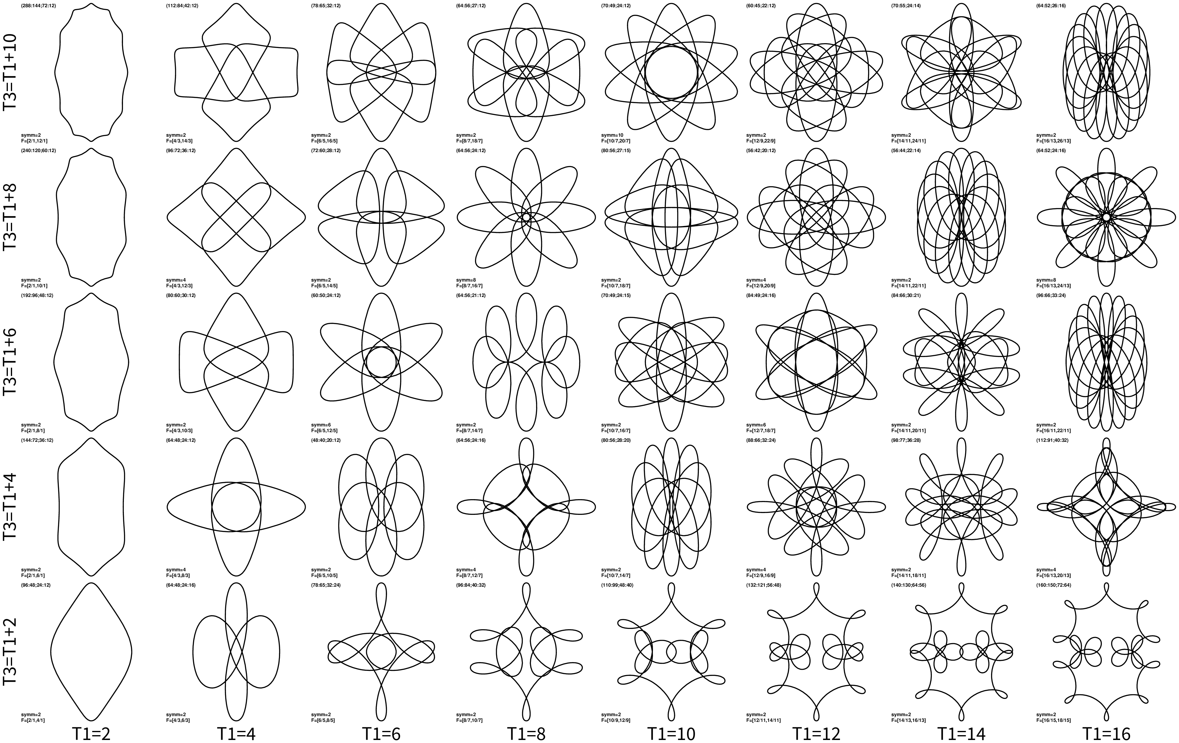
And nsymm=4:
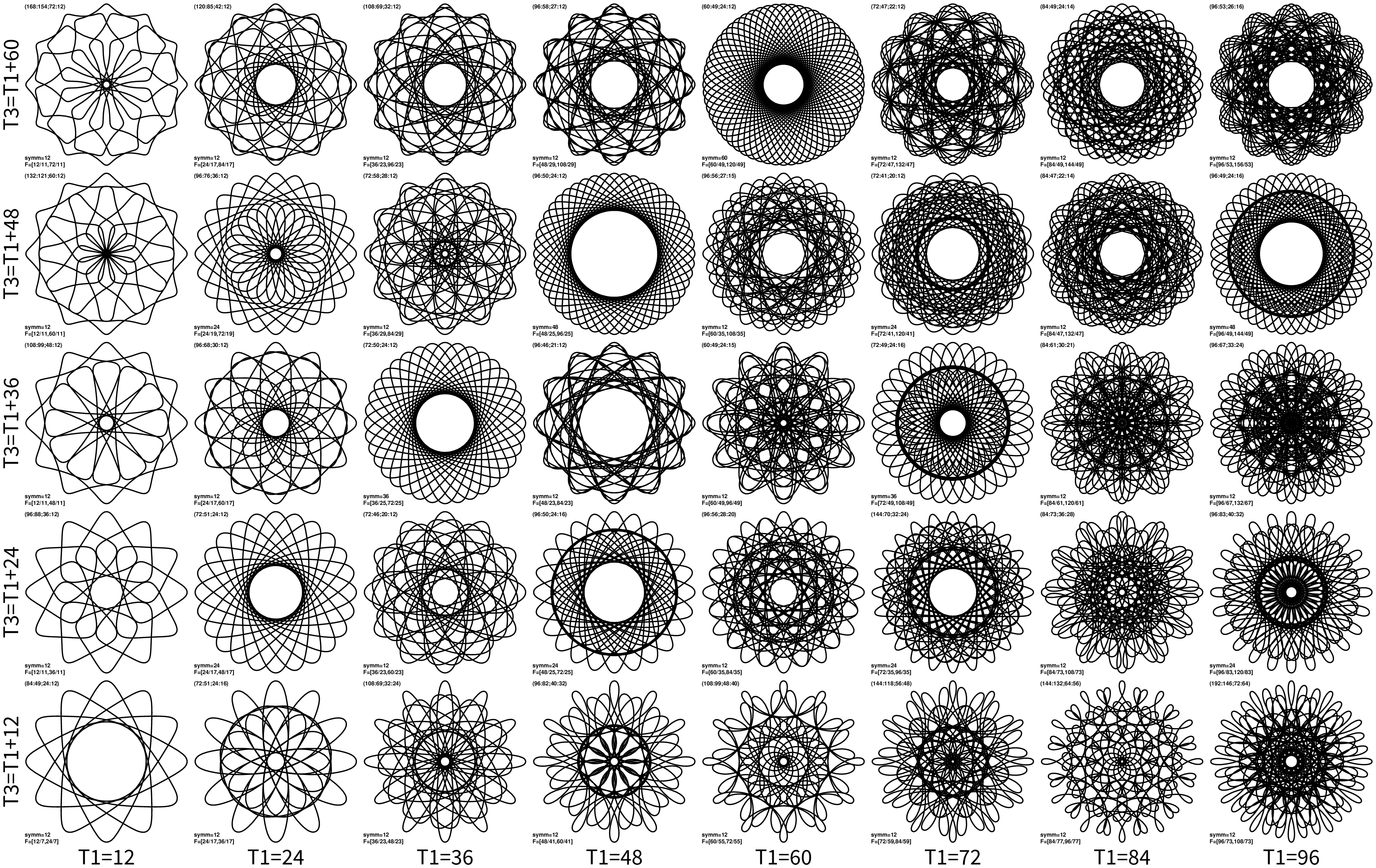
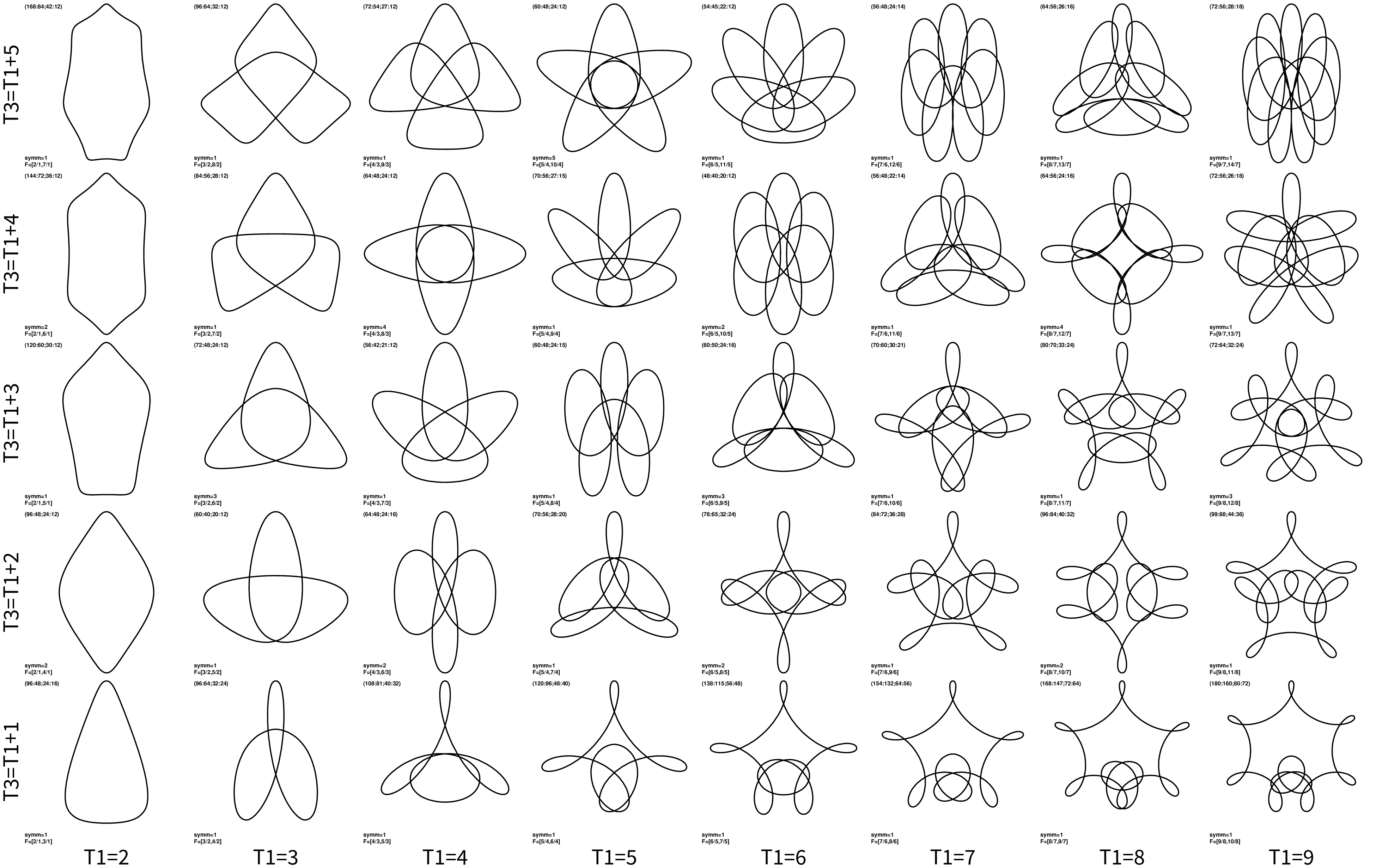
I will give here links to other grids: nsymm=12, nsymm=11, nsymm=10, nsymm=9, nsymm=8, nsymm=6, nsymm=3, nsymm=2, nsymm=1,
One has to remember that these 2D grids are still a small slice of all possibilities: each panel represents many other curves that have same T1 and T3, but different T. Most will be boring (“ropy” pattern, …), but some might have lines spread in different, maybe more pleasing, way. Still, they should be in a way similar to the displayed panels (check previous article for an example cut along T).
Also a useful information is that on average my code was finding T values (zoom into images to read small legend next to each panel) that are very close to about T≈0.8T1. Another detail that might be needed to reproduce the plots: during the frequency inversion one can choose integers a and b in different ways, and my code prefers values that make n1≈2n2, which in turn allows hoop separation h of about 0.5.